Quantum algorithms on the Xanadu quantum cloud

In this tutorial, we program photonic devices available on the Xanadu cloud platform to implement proof-of-principle algorithms for Gaussian boson sampling, molecular vibronic spectra, and graph similarity. You will learn how to use Strawberry Fields 🍓 to program the chips and process the output samples for each task. We follow closely the results presented in the paper “Quantum circuits with many photons on a programmable nanophotonic chip” [1].

More details on how to submit jobs to the Xanadu cloud can be found in this tutorial. Additional information on the algorithms themselves can be found in the tutorials for vibronic spectra and graph similarity.

Finally, an authentication token is required to access hardware ️🔑. If you do not have an authentication token, please sign up for hardware access via Xanadu Cloud.

Remote programming of photonic chips

Strawberry Fields is a software platform for photonic quantum computing — it provides access to tools for designing and simulating photonic circuits, and also serves as the application programming interface for photonic hardware on the Xanadu cloud. In this tutorial, we program X8 devices, which consist of eight modes separated into four spatial modes, each carrying two separate frequencies. We call modes 0 to 3 the signal modes and modes 4 to 7 the idler modes.

The circuit architecture consists of the following components:

• Firstly, two mode squeezing operations act on each pair of signal/idler modes. Squeezing can be turned on or off for a fixed squeezing level.

• The second component of the circuit is a universal four-mode interferometer acting equally on signal and idler modes.

• Finally, output modes are probed using transition-edge sensors capable of counting the number of photons.

The figure below shows a micrograph of the chip, a photograph of the complete system fit to a standard server rack, and a schematic of the control system.

Gaussian boson sampling

Gaussian boson sampling is a platform for photonic quantum computing where a Gaussian state is measured in the photon-number basis. The combinations of squeezing and interferometer operations implemented in Xanadu’s hardware generate a Gaussian output state, so these devices can be used to implement Gaussian boson sampling. When the interferometers are programmed according to random unitaries, arguments from computational complexity theory can be invoked to argue that the output distribution cannot be sampled from efficiently using classical computers.

Haar-random unitaries can be generated using the random_interferometer() function.

from strawberryfields.utils import random_interferometer
U_GBS = random_interferometer(4)

We define a program on eight modes where two-mode squeezing gates are applied to each pair of signal-idler modes. To maximize the number of photons generated, we turn all squeezers on and program the interferometer according to the random unitary generated above.

import strawberryfields as sf
from strawberryfields import ops

nr_modes = 8
gbs_prog = sf.Program(nr_modes)
with gbs_prog.context as q:
    # Two-mode squeezing. Allowed values are r=1.0 (on) or r=0.0 (off)
    ops.S2gate(1.0) | (q[0], q[4])
    ops.S2gate(1.0) | (q[1], q[5])
    ops.S2gate(1.0) | (q[2], q[6])
    ops.S2gate(1.0) | (q[3], q[7])

    # Equal interferometers on signal and idler modes
    ops.Interferometer(U_GBS) | (q[0], q[1], q[2], q[3])
    ops.Interferometer(U_GBS) | (q[4], q[5], q[6], q[7])

    # Measure output state in the Fock basis
    ops.MeasureFock() | q

This program can then be executed across any compatible device. We run the remote engine to request 400,000 samples (four hundred thousand samples! 🤯) from Xanadu’s X8 chip.

from strawberryfields import RemoteEngine

eng = sf.RemoteEngine("X8")
gbs_results = eng.run(gbs_prog, shots=400000)
gbs_samples = gbs_results.samples

To visualize the results, we create a histogram depicting the probabilities of observing all possible patterns with four photons. These can be arranged into orbits that describe how the photons are distributed across modes. For example the orbit \([1, 1, 1, 1]\) is the set of all patterns where a single photon is detected in four different modes, e.g., \([0, 1, 1, 0, 0, 1, 0, 1]\). Similarly the orbit \([2, 2]\) is the set of all patterns where two photons are detected in one mode and two photons are detected in another mode, e.g., \([0, 0, 2, 0, 2, 0, 0, 0]\).

from sympy.utilities.iterables import multiset_permutations
from strawberryfields.apps.similarity import orbits
import numpy as np

nr_photons = 4

# generate all possible patterns and count the number in each orbit
patterns = []
counts = []
counter = 0
for orb in orbits(nr_photons):
    orb = orb + [0] * (nr_modes - len(orb))
    for p in multiset_permutations(orb):
        patterns.append(p)
        counter += 1
    counts.append(counter)

patterns = np.array(patterns)
nr_patterns = len(patterns)

print(list(orbits(nr_photons)))
print(counts)

Out:

[[1, 1, 1, 1], [2, 1, 1], [3, 1], [2, 2], [4]]
[70, 238, 294, 322, 330]

To create the histogram, we use a python dictionary that assigns a unique number to each pattern, making it easy to record the number of times each pattern is observed.

sample_dict = {}
for i in range(nr_patterns):
    sample_dict[str(patterns[i])] = i

We iterate over all samples with four photons, keeping track of the number of times each pattern appears. The resulting array is normalized so its entries sum to unity. This provides an empirical estimate of the conditional probability of observing each pattern across samples with four photons.

from strawberryfields.apps.sample import postselect

# post-select samples on outputs with four photons
gbs_samples = postselect(gbs_samples, nr_photons, nr_photons)

probs_samples = np.zeros(nr_patterns)

for s in gbs_samples:
    index = sample_dict[str(s)]
    probs_samples[index] += 1

norm = np.sum(probs_samples)
probs_samples = np.array([p / norm for p in probs_samples])

We plot the reconstructed probability distribution. We use a different colour for each of the five orbit of four photons: \([1,1,1,1]\), \([2,1,1]\), \([3,1]\), \([2,2]\), \([4]\). The resulting histogram depicts that some patterns occur with higher probability than others.

import matplotlib.pyplot as plt

plt.figure()
x = np.arange(nr_patterns)
plt.bar(x[:counts[0]], probs_samples[:counts[0]], color="#508104")
plt.bar(x[counts[0]:counts[1]], probs_samples[counts[0]:counts[1]], color="#9e8e01")
plt.bar(x[counts[1]:counts[2]], probs_samples[counts[1]:counts[2]], color="#f3b800")
plt.bar(x[counts[2]:counts[3]], probs_samples[counts[2]:counts[3]], color="#db8200")
plt.bar(x[counts[3]:counts[4]], probs_samples[counts[3]:counts[4]], color="#b64201")
plt.xlabel("Pattern")
plt.xticks([], [])
plt.ylabel("Probability")
plt.show()

Vibronic spectra

Molecules can absorb light when they undergo a transition between different vibrational and electronic (vibronic) states. The vibronic spectrum of a molecule describes the wavelengths of light that are more strongly absorbed in this process. In the photonic algorithm for vibronic spectra, optical modes represent the vibrational normal modes of the molecule. The device is programmed to replicate the transformation experienced by the vibrational modes during a vibronic transition.

In this proof-of-principle demonstration, we program the device according to the interferometer transformations that result from the mode-mixing of ethylene upon a vibronic transition. This interferometer is described by the following unitary:

U_vibronic = np.array([
    [-0.5349105592386603, 0.8382670887228271, 0.10356058421030308, -0.021311662937477004],
    [-0.6795134137271818, -0.4999083619063322, 0.5369830827402383, 0.001522863010877817],
    [-0.4295084785810517, -0.17320833713971984, -0.7062800928050401, 0.5354341876268153],
    [0.2601051345260338, 0.13190447151471643, 0.4495473331653913, 0.8443066531962792]
])

We define a new program to execute the vibronic spectrum algorithm. We only include squeezing on the first pair of modes.

eng = sf.RemoteEngine("X8")
vibronic_prog = sf.Program(nr_modes)

with vibronic_prog.context as q:
    ops.S2gate(1.0) | (q[0], q[4])

    ops.Interferometer(U_vibronic) | (q[0], q[1], q[2], q[3])
    ops.Interferometer(U_vibronic) | (q[4], q[5], q[6], q[7])

    ops.MeasureFock() | q

vibronic_results = eng.run(vibronic_prog, shots=400000)
vibronic_samples = vibronic_results.samples

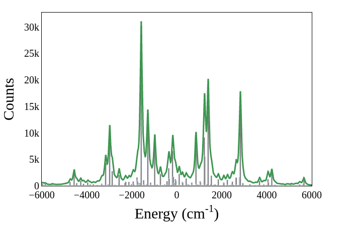
The Strawberry Fields applications module contains functionality for reconstructing vibronic spectra. Each photon pattern is assigned an energy that can be used to reconstruct a histogram. The peaks of this histogram represent the absorption lines of the molecule’s vibronic spectrum. We employ a convention where zero energy is assigned to a transition between vibrational ground states of the initial and final electronic states, which correspond to vacuum outputs.

from strawberryfields.apps import vibronic, plot
import plotly

vibronic_samples = [list(s) for s in vibronic_samples]

# frequencies of the initial and final normal modes
w = [2979, 1580, 1286, 977]
wp = [2828, 1398, 1227, 855]
energies = vibronic.energies(vibronic_samples, w, wp)
plot.spectrum(energies, xmin=-6000, xmax=6000)

Graph similarity

Graphs can be encoded in photonic circuits by selecting squeezing values and interferometer settings according to a decomposition of the graph’s adjacency matrix. The statistics of the resulting distribution of photon patterns carry information about the encoded graph, which can be used to study similarity between graphs. One method to achieve this is to estimate orbit probabilities and collect them in the form of feature vectors.

The specific architecture of X8 chips permits the encoding of bipartite weighted graphs such that the non-zero eigenvalues of their adjacency matrix are all equal. The adjaceny matrices of bipartite graphs have block structure, where the off-diagonal blocks contain the edge weights connecting nodes in the separate bipartitions.

We construct two such adjacency matrices A1 and A2 from the respective off-diagonal blocks C1 and C2:

# off-diagonal blocks
C1 = np.array(
    [
        [0.0826, 0.1231, 0.0789, -0.1969],
        [0.1231, 0.1834, 0.1176, -0.2935],
        [0.0789, 0.1176, 0.0754, -0.1882],
        [-0.1969, -0.2935, -0.1882, 0.4697],
    ]
)

C2 = np.array(
    [
        [0.7925, 0.1076, -0.0125, 0.0545],
        [0.1076, 0.1869, 0.0725, -0.3160],
        [-0.0125, 0.0725, 0.8026, 0.0367],
        [0.0545, -0.3160, 0.0367, 0.6511],
    ]
)

# full adjacency matrices
O = np.zeros((4, 4))
A1 = np.block([[O, C1], [C1.T, O]])
A2 = np.block([[O, C2], [C2.T, O]])

The squeezing parameters \(r_i\) and interferometer unitary \(U\) of the circuit encoding the graphs are related to the Autonne-Takagi decomposition of the off-diagonal blocks \(C\) as \(C = U\,\text{diag}(r_i)\,U^T\). These parameters can be obtained directly using Strawberry Fields.

r1, U1 = sf.decompositions.takagi(C1)
r2, U2 = sf.decompositions.takagi(C2)

print(r1)
print(r2)

Out:

[8.11073932e-01 7.01706638e-05 3.67973142e-05 7.30565705e-06]
[8.11092959e-01 8.11039956e-01 8.11020979e-01 5.38942155e-05]

To convert into a format accepted by the device, we set negligible values to zero and others equal to one, i.e., we turn on squeezers corresponding to non-negligible values. This results simply in changing the total mean photon number of the distribution.

# set small values to zero
r1[np.abs(r1) < 1e-2] = 0.0
r2[np.abs(r2) < 1e-2] = 0.0

# set large values to one
r1[np.abs(r1) > 1e-2] = 1.0
r2[np.abs(r2) > 1e-2] = 1.0

# first graph
eng = sf.RemoteEngine("X8")
similarity_prog1 = sf.Program(nr_modes)

with similarity_prog1.context as q:
    for i, r in enumerate(r1):
        ops.S2gate(r) | (q[i], q[i + 4])

    ops.Interferometer(U1) | (q[0], q[1], q[2], q[3])
    ops.Interferometer(U1) | (q[4], q[5], q[6], q[7])
    ops.MeasureFock() | q

similarity_results1 = eng.run(similarity_prog1, shots=400000)
similarity_samples1 = similarity_results1.samples

# second graph
eng = sf.RemoteEngine("X8")
similarity_prog2 = sf.Program(nr_modes)

with similarity_prog2.context as q:
    for i, r in enumerate(r2):
        ops.S2gate(r) | (q[i], q[i + 4])

    ops.Interferometer(U2) | (q[0], q[1], q[2], q[3])
    ops.Interferometer(U2) | (q[4], q[5], q[6], q[7])
    ops.MeasureFock() | q

similarity_results2 = eng.run(similarity_prog2, shots=400000)
similarity_samples2 = similarity_results2.samples

We create feature vectors whose entries are given by the probabilities of observing samples inside different orbits. We consider the simple case of three-dimensional feature vectors constructed from orbits of three, four, and five photons. These can be obtained directly using Strawberry Fields.

from strawberryfields.apps.similarity import feature_vector_orbits_sampling

orbits = [[1, 1, 1], [1, 1, 1, 1], [2, 1, 1, 1]]
vector1 = feature_vector_orbits_sampling(similarity_samples1, orbits)
vector2 = feature_vector_orbits_sampling(similarity_samples2, orbits)

We plot the feature vectors, which reflect and quantify the degree of similarity between their corresponding graphs.

fig = plt.figure()
ax = fig.add_subplot(111, projection='3d')

ax.scatter(vector1[0], vector1[1], vector1[2], color="#508104", s=150)
ax.scatter(vector2[0], vector2[1], vector2[2], color="#b64201", s=150)
ax.set_xlabel('[1, 1, 1]')
ax.set_ylabel('[1, 1, 1, 1]')
ax.set_zlabel('[2, 1, 1, 1]')

plt.show()

Conclusion

The demonstrations covered in this tutorial are photonic quantum algorithms executed remotely on programmable nanophotonic devices. There is something remarkable about this statement. It was not long ago that all quantum optics experiments occurred on large optical tables that could only be configured by a handful of experts familiar with the experimental setup. Technological progress across integrated nanophotonics, quantum software, and quantum algorithm development have made it possible for researchers and enthusiasts around the world to perform experiments from the comfort of their homes using just a few lines of code. We look forward to seeing what the community will be able to achieve when they play with these new toys. 😊

References

1

J.M. Arrazola, V. Bergholm, K. Brádler, T.R. Bromley, M.J. Collins, I. Dhand, A. Fumagalli, T. Gerrits, A. Goussev, L.G. Helt, J. Hundal, T. Isacsson, R.B. Israel, J. Izaac, S. Jahangiri, R. Janik, N. Killoran, S.P. Kumar, J. Lavoie, A.E. Lita, D.H. Mahler, M. Menotti, B. Morrison, S.W. Nam, L. Neuhaus, H.Y. Qi, N. Quesada, A. Repingon, K.K. Sabapathy, M. Schuld, D. Su, J. Swinarton, A. Száva, K. Tan, P. Tan, V.D. Vaidya, Z. Vernon, Z. Zabaneh, Y. Zhang, Nature, 591, 54-60, (2021).

demos/tutorial_X8_demos

 

Download Python script

 

Download Notebook