Theory
The following pages can be used to gain an understanding of photonic quantum computing. Explore near-term photonic devices, learn about the theory underpinning photonic quantum computers, and check out our reference pages of photonic computing conventions and formulas.
Introduction to quantum photonics
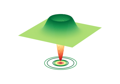
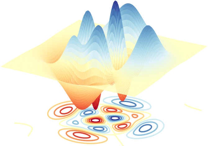
Photonic quantum systems are described by a slightly different model than qubits. The basic elements of a photonic system are qumodes, each of which can be described by a superposition over different numbers of photons. This model leads to a different set of quantum gates and measurements.
In the long term, the photonic and qubit-based approaches will be able to run the same set of established quantum algorithms. On the other hand, near-term photonic and qubit systems will excel at their own specific tasks.
Read more to get to grips with the photonic model of quantum computing and see how it contrasts with the qubit model.
Read more
Gaussian boson sampling
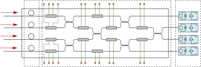
The near-term devices available for photonic quantum computing has a fixed architecture with controllable gates. This architecture realizes an algorithm known as Gaussian boson sampling (GBS), which can be programmed to solve a range of practical tasks in graphs and networking, machine learning, chemistry (see Applications for more details on practical applications).
A GBS device can be programmed to embed any symmetric matrix. Read more for further details on GBS without needing to dive deeper into quantum computing!
Read more
Conventions and formulas
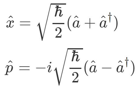
Describing a quantum system requires a number of conventions to be fixed, including the value of Planck’s constant \(\hbar\) (we set \(\hbar=2\) by default).
This section details formulas and constants used throughout Strawberry Fields and can be used for reference when constructing quantum circuits.
Contents
Downloads
Related tutorials