Note
Click here to download the full example code
Executing programs on X8 devices
In this tutorial, we demonstrate how Strawberry Fields can execute quantum programs on the X8 family of remote photonic devices, via the Xanadu cloud platform. Topics covered include:
Configuring Strawberry Fields to access the cloud platform,
Using the
RemoteEngineto execute jobs remotely onX8,Compiling quantum programs for specific quantum chip architectures,
Saving and running Blackbird scripts, an assembly language for quantum photonic hardware, and
Embedding and sampling from bipartite graphs on
X8.
Warning
An API key is required to access the Xanadu Cloud platform locally. In the following,
replace AUTHENTICATION_TOKEN with your personal API token.
If you do not have an API key, you can contact us to setup an account.
Note
What’s in a name?
X8, rather than being a single hardware chip, corresponds to a family of physical devices,
with individual names including X8_01.
While X8 is used here to specify any chip in the X8 device class (including
X8_01), you may also specify a specific chip ID (such as X8_01) during program
compilation and execution.
Configuring your credentials
Before using RemoteEngine for the first time, we need to register
a Xanadu Cloud API key with the Xanadu Cloud Client (XCC). We can do this by using the
xcc.Settings class from the XCC.
import xcc
xcc.Settings(REFRESH_TOKEN="Xanadu Cloud API key goes here").save()
This only needs to be executed once; your Xanadu Cloud credentials will be saved to disk
and automatically loaded when a new RemoteEngine instance is created.
To test that your account credentials correctly authenticate against the cloud platform,
you can import xcc.commands and use the xcc.commands.ping() command,
import xcc.commands
xcc.commands.ping()
Out:
'Successfully connected to the Xanadu Cloud.'
Note
The XCC also provides a command line interface for configuring access to the cloud platform and for submitting jobs:
$ xcc config set REFRESH_TOKEN "Xanadu Cloud API key goes here"
$ xcc ping
Successfully connected to the Xanadu Cloud.
For more details on configuring Strawberry Fields for cloud access, including using the command line interface, see the Hardware and cloud quickstart guide.
Device details
Below, we will be submitting a job to run on X8.
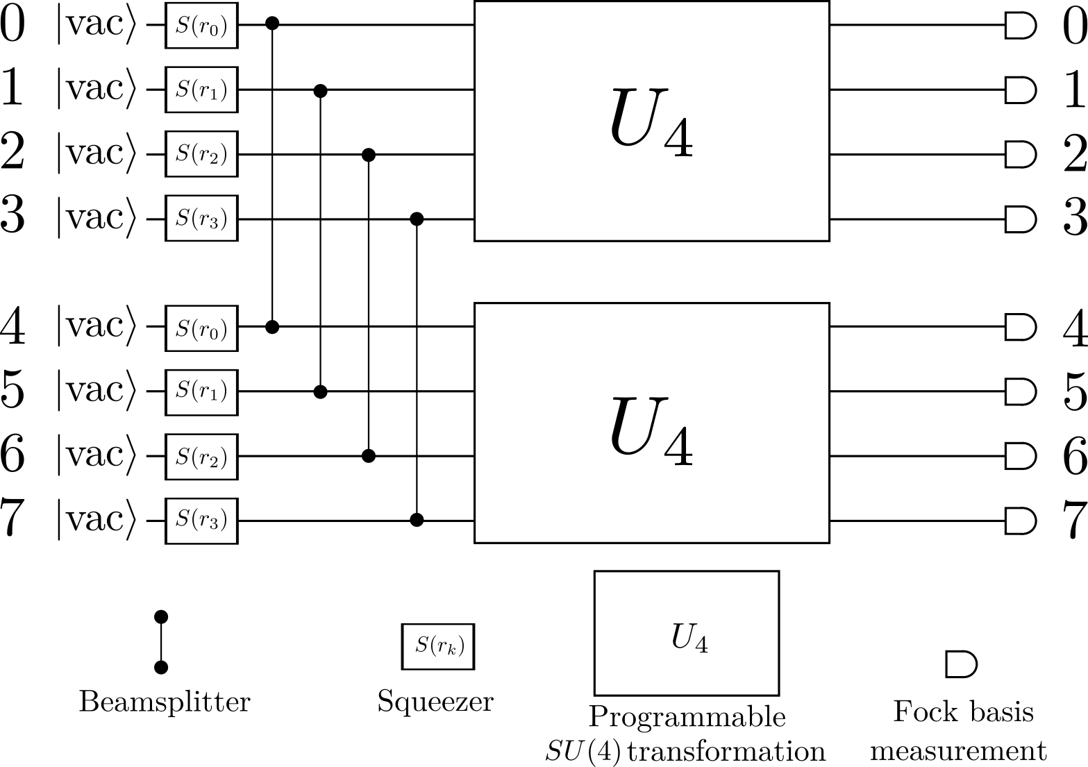
X8 is an 8-mode chip, with the following restrictions:
The initial states are two-mode squeezed states (
S2gate). We call modes 0 to 3 the signal modes and modes 4 to 7 the idler modes. Two-mode squeezing is between the pairs of modes: (0, 4), (1, 5), (2, 6), (3, 7).Any arbitrary \(4\times 4\) unitary (consisting of
BSgate,MZgate,Rgate, andInterferometeroperations) can be applied identically on both the signal and idler modes.Finally, the chip terminates with photon-number resolving measurements (
MeasureFock).
At this point, only the parameters (r=1, phi=0) and (r=0, phi=0) (corresponding to no
squeezing) are allowed for the two-mode squeezing gates between any pair of signal and idler
modes. Eventually, a range of squeezing amplitudes r will be supported.
Executing jobs
In this section, we will use Strawberry Fields to submit a simple circuit to the chip.
First, we import NumPy and Strawberry Fields, including the remote engine.
import numpy as np

import strawberryfields as sf
from strawberryfields import ops
from strawberryfields import RemoteEngine
Lets use the random_interferometer() function to generate a random \(4\times 4\)
unitary:
from strawberryfields.utils import random_interferometer
U = random_interferometer(4)
np.set_printoptions(precision=16)
print(U)
Out:
array([[-0.2075958002056761-0.1295303874004949j, 0.4168590195887626+0.585773678107707j, 0.2890475539846776-0.3529463027479843j, 0.213901659507021 +0.411521709357663j ],
[-0.2618964139102731+0.4432947111670047j, -0.5184820552871022+0.1650915362584557j, -0.4128306651379415-0.4882838386727423j, -0.0079437590004708+0.172938838723708j ],
[ 0.1415402337953751+0.5501271526107689j, 0.3692746956219556+0.0108433797647406j, 0.1986531501150634-0.1359201690880894j, -0.6937372152789114-0.0404525424120204j],
[-0.5917850330700981-0.0462912812620793j, 0.1868543708455093-0.1249918525715507j, -0.322811013686639 +0.4699849324731709j, -0.2704622309566428+0.4459455876188795j]])
Next we create an 8-mode quantum program:
prog = sf.Program(8, name="remote_job1")

with prog.context as q:
    # Initial squeezed states
    # Allowed values are r=1.0 or r=0.0
    ops.S2gate(1.0) | (q[0], q[4])
    ops.S2gate(1.0) | (q[1], q[5])
    ops.S2gate(1.0) | (q[3], q[7])

    # Interferometer on the signal modes (0-3)
    ops.Interferometer(U) | (q[0], q[1], q[2], q[3])
    ops.BSgate(0.543, 0.123) | (q[2], q[0])
    ops.Rgate(0.453) | q[1]
    ops.MZgate(0.65, -0.54) | (q[2], q[3])

    # *Same* interferometer on the idler modes (4-7)
    ops.Interferometer(U) | (q[4], q[5], q[6], q[7])
    ops.BSgate(0.543, 0.123) | (q[6], q[4])
    ops.Rgate(0.453) | q[5]
    ops.MZgate(0.65, -0.54) | (q[6], q[7])

    ops.MeasureFock() | q
Finally, we create the engine. Similarly to the LocalEngine, the
RemoteEngine is in charge of compiling and executing programs. However,
it differs in that the program will be executed on remote devices, rather than on local
simulators.
Below, we create a remote engine to submit and execute quantum programs
on the X8 photonic device.
eng = RemoteEngine("X8")
We can now run the program by calling eng.run, and passing the program to be executed
as well as additional runtime options.
results = eng.run(prog, shots=20)
Out:
2022-03-22 15:48:31,995 - INFO - Compiling program for device X8_01 using compiler Xunitary.
2022-03-22 15:48:52,487 - INFO - The remote job 0884466f-b0f1-4153-8b8f-5f0b7ff9e8fd has been completed.
print(results.samples)
Out:
array([[0, 0, 1, 0, 1, 0, 1, 0],
       [0, 0, 0, 0, 0, 0, 0, 0],
       [0, 0, 0, 0, 0, 0, 0, 2],
       [0, 0, 0, 0, 0, 1, 0, 0],
       [1, 0, 0, 0, 0, 0, 3, 0],
       [3, 0, 0, 0, 2, 0, 1, 0],
       [0, 1, 0, 0, 0, 1, 1, 0],
       [0, 1, 0, 0, 1, 0, 0, 0],
       [0, 0, 0, 0, 0, 0, 1, 1],
       [0, 0, 0, 0, 0, 0, 0, 0],
       [0, 0, 0, 0, 0, 1, 0, 0],
       [1, 0, 0, 0, 1, 0, 0, 0],
       [0, 0, 0, 0, 0, 0, 1, 0],
       [0, 0, 0, 0, 0, 0, 0, 0],
       [0, 0, 0, 0, 0, 0, 0, 1],
       [0, 0, 0, 0, 0, 0, 0, 1],
       [1, 0, 0, 0, 0, 0, 0, 0],
       [0, 0, 0, 0, 0, 1, 0, 0],
       [0, 0, 1, 1, 0, 2, 1, 2],
       [2, 0, 1, 0, 1, 0, 0, 0]])
The samples returned correspond to 20 measurements (or shots) of the 8 mode quantum program above. Some modes have measured zero photons, and others have detected single photons, with a few even detecting 2 or 3.
By taking the average of the returned array along the shots axis, we can estimate the mean photon number of each mode:
print(np.mean(results.samples, axis=0))
Out:
array([0.4, 0.1, 0.15, 0.05, 0.3, 0.3, 0.45, 0.35])
We can also use the Python collections module to convert the samples into counts:
from collections import Counter
bitstrings = [tuple(i) for i in results.samples]
counts = {k:v for k, v in Counter(bitstrings).items()}
print(counts[(0, 0, 0, 0, 0, 0, 0, 0)])
Out:
2
Note
The operation decorator allows you to create your own
Strawberry Fields operation. This can make it easier to ensure that the same unitary is always
applied to the signal and idler modes.
from strawberryfields.utils import operation

@operation(4)
def unitary(q):
    ops.Interferometer(U) | q
    ops.BSgate(0.543, 0.123) | (q[2], q[0])
    ops.Rgate(0.453) | q[1]
    ops.MZgate(0.65, -0.54) | (q[2], q[3])

prog = sf.Program(8)

with prog.context as q:
    ops.S2gate(1.0) | (q[0], q[4])
    ops.S2gate(1.0) | (q[1], q[5])
    ops.S2gate(1.0) | (q[3], q[7])

    unitary() | q[:4]
    unitary() | q[4:]

    ops.MeasureFock() | q
Refer to the operation documentation for more details.
Job management
Above, when we called eng.run(), we had to wait for the
remote device to execute the program and the result to be returned before we could
continue executing code. That is, eng.run() is a blocking method.
Sometimes, however, it is useful to submit the program
and continue performing computation locally, every now and again checking to see
if the job is complete and the results are ready. This is possible with
the non-blocking eng.run_async() method:
job = eng.run_async(prog, shots=100)
Unlike eng.run(), it returns a xcc.Job instance, which allows us to
check the status of our submitted job:
print(job.id)
print(job.status)
Out:
"4c734d7b-6d9e-4df0-9e18-19356a66123d"
"queued"
When the job result is ready, it is available via the result property. To
update the status of the job, job.clear() can be called. This will clear
the cached property values of the job and re-fetch them when they’re called again.
job.clear()
job.status()
Out:
"queued"
Instead of clearing the cache and checking the status, job.wait() can be
called. This is a blocking method which automatically refreshes and checks the status of the
job. Once the job is finished it will continue executing the next line.
job.wait()
print(job.status)
Out:
"complete"
The returned result from the xcc.Job object will be a dictionary containing the samples
under the first entry of the “output” key. We can encapsulate the data in an sf.Result object, which is the type of the object returned by the eng.run()
method above.
result = sf.Result(job.result)
print(result.samples.shape)
Out:
(100, 8)
Finally, an incomplete job can be cancelled by calling job.cancel().
Hardware compilation
When creating a quantum program to run on hardware, Strawberry Fields can compile any collection of the following gates into a multi-mode unitary:
Furthermore, several automatic decompositions are supported:
You can use the
Interferometercommand to directly pass a unitary matrix to be decomposed and compiled to match the device architecture. This performs a rectangular decomposition using Mach-Zehnder interferometers.You can use
BipartiteGraphEmbedto embed a bipartite graph on the photonic device.Warning
Decomposed squeezing values depend on the graph structure, so only bipartite graphs that result in equal squeezing on all modes can be executed on
X8chips. This restriction will be lifted in the future with new generations of chip.
Before sending the program to the cloud platform to be executed, however, Strawberry Fields must
compile the program to match the physical architecture or layout of the photonic chip, in this
case X8. This happens implicitly when using the remote engine, however we can use the
compile() method to explicitly compile the program for a specific chip.
For example, lets compile the program we created in the previous section.
To do so we make use of the eng.device object containing hardware-related information for the
compilation and validation of programs.
prog_compiled = prog.compile(device=eng.device)
prog_compiled.print()
Out:
S2gate(1, 0) | (q[0], q[4])
S2gate(1, 0) | (q[1], q[5])
S2gate(0, 0) | (q[2], q[6])
S2gate(1, 0) | (q[3], q[7])
MZgate(0.6666, 5.766) | (q[0], q[1]
MZgate(1.977, 3.391) | (q[2], q[3])
MZgate(1.138, 1.928) | (q[1], q[2])
MZgate(1.531, 1.561) | (q[0], q[1])
MZgate(0.9116, 0.5838) | (q[2], q[3])
MZgate(2.462, 1.365) | (q[1], q[2])
Rgate(1.353) | (q[0])
Rgate(5.833) | (q[1])
Rgate(2.993) | (q[2])
Rgate(0.5873) | (q[3])
MZgate(0.6666, 5.766) | (q[4], q[5])
MZgate(1.977, 3.391) | (q[6], q[7])
MZgate(1.138, 1.928) | (q[5], q[6])
MZgate(1.531, 1.561) | (q[4], q[5])
MZgate(0.9116, 0.5838) | (q[6], q[7])
MZgate(2.462, 1.365) | (q[5], q[6])
Rgate(1.353) | (q[4])
Rgate(5.833) | (q[5])
Rgate(2.993) | (q[6])
Rgate(0.5873) | (q[7])
MeasureFock | (q[0], q[1], q[2], q[3], q[4], q[5], q[6], q[7])
While equivalent to the uncompiled program, we can now see the low-level hardware operations that are applied on the physical chip.
Note
By default, the device specification will instruct Strawberry Fields which compilation strategy to apply. However, the compiler strategy can be explicitly provided in addition to the device specification:
>>> prog2 = prog.compile(device=device, compiler="Xunitary")
While some compilers may require a device spec, they can also be used independently:
>>> prog2 = prog.compile(compiler="Xunitary")
For more details on available compilers, see Circuits.
Working with Blackbird scripts
When submitting quantum programs to be executed remotely, they are communicated to
the cloud platform using Blackbird—a quantum photonic assembly language.
Strawberry Fields also supports exporting programs directly as Blackbird scripts
(an xbb file); Blackbird scripts can then be submitted to be executed via the
Xanadu Cloud Client.
For example, lets consider a Blackbird script program1.xbb
representing the same quantum program we constructed above:
name remote_job1
version 1.0
target X8_01 (shots = 20)

# Initial states are two-mode squeezed states
S2gate(1.0, 0.0) | [0, 4]
S2gate(1.0, 0.0) | [1, 5]
S2gate(0.0, 0.0) | [2, 6]
S2gate(1.0, 0.0) | [3, 7]

# Apply the compiled MZgates and Rgates from
# above to the signal modes
MZgate(0.6665938628222643, 5.765809053658708) | [0, 1]
MZgate(1.9765338789427835, 3.3911669348390467) | [2, 3]
MZgate(1.138222372780161, 1.9282663401816624) | [1, 2]
MZgate(1.531178005879373, 1.5605970765345907) | [0, 1]
MZgate(0.9115589243094834, 0.5838121565893191) | [2, 3]
MZgate(2.462416459243228, 1.3645885573522776) | [1, 2]
Rgate(1.3525981148291777) | 0
Rgate(5.832982291650049) | 1
Rgate(2.993152273515084) | 2
Rgate(0.5872963359911774) | 3

# Apply the compiled MZgates and Rgates from
# above to the idler modes
MZgate(0.6665938628222643, 5.765809053658708) | [4, 5]
MZgate(1.9765338789427835, 3.3911669348390467) | [6, 7]
MZgate(1.138222372780161, 1.9282663401816624) | [5, 6]
MZgate(1.531178005879373, 1.5605970765345907) | [4, 5]
MZgate(0.9115589243094834, 0.5838121565893191) | [6, 7]
MZgate(2.462416459243228, 1.3645885573522776) | [5, 6]
Rgate(1.3525981148291777) | 4
Rgate(5.832982291650049) | 5
Rgate(2.993152273515084) | 6
Rgate(0.5872963359911774) | 7

# Perform a PNR measurement in the Fock basis
MeasureFock() | [0, 1, 2, 3, 4, 5, 6, 7]
The above Blackbird script can be remotely executed using the command line,
$ xcc job submit --name "remote_job1" --target "X8_01" --circuit "$(cat program1.xbb)"
Out:
{
    "id": "743bad0a-8a21-4a6b-86de-50f7ff35a9b3",
    "name": "remote_job1",
    "status": "open",
    "target": "X8_01",
    "language": "blackbird:1.0",
    "created_at": "2021-11-16 21:15:50.257162+00:00",
    "finished_at": null,
    "running_time": null,
    "metadata": {}
}
Warning
Windows PowerShell users should write Get-Content remote_job1.xbb -Raw instead of cat program1.xbb.
After executing the above command, the result will be accessible via its unique ID
$ xcc job get 743bad0a-8a21-4a6b-86de-50f7ff35a9b3 --result
Embedding bipartite graphs
The X8 device class supports embedding bipartite graphs, i.e., those with adjacency matrices
where \(B\) represents the edges between the two sets of vertices in the graph. However, the devices are currently restricted to bipartite graphs with equally sized partitions, such that the singular values form the set \(\{0, d\}\) for some real value \(d\).
Here, we will consider a complete bipartite graph, since the singular values are of the form \(\{0, d\}\).
B = np.ones([4, 4])
A = np.block([[0*B, B], [B.T, 0*B]])

prog = sf.Program(8)

# the following mean photon number per mode
# quantity is set to ensure that the singular values
# are scaled such that all Sgates have squeezing value r=1
m = 0.345274461385554870545

with prog.context as q:
    ops.BipartiteGraphEmbed(A, mean_photon_per_mode=m) | q
    ops.MeasureFock() | q


prog.compile(device=eng.device).print()
Out:
S2gate(1, 0) | (q[0], q[4])
S2gate(0, 0) | (q[3], q[7])
S2gate(0, 0) | (q[2], q[6])
MZgate(3.598, 5.444) | (q[2], q[3])
MZgate(3.598, 5.444) | (q[6], q[7])
S2gate(0, 0) | (q[1], q[5])
MZgate(0, 5.236) | (q[0], q[1])
MZgate(4.886, 5.496) | (q[1], q[2])
MZgate(0.7106, 4.492) | (q[2], q[3])
Rgate(0.9284) | (q[3])
MZgate(2.922, 3.142) | (q[0], q[1])
MZgate(4.528, 3.734) | (q[1], q[2])
Rgate(-2.51) | (q[2])
MZgate(0, 5.236) | (q[4], q[5])
MZgate(4.886, 5.496) | (q[5], q[6])
MZgate(0.7106, 4.492) | (q[6], q[7])
Rgate(0.9284) | (q[7])
MZgate(2.922, 3.142) | (q[4], q[5])
MZgate(4.528, 3.734) | (q[5], q[6])
Rgate(-2.51) | (q[6])
Rgate(-2.51) | (q[1])
Rgate(-0.8273) | (q[4])
Rgate(-0.8273) | (q[0])
Rgate(-2.51) | (q[5])
MeasureFock | (q[0], q[1], q[2], q[3], q[4], q[5], q[6], q[7])
If the bipartite graph to be embedded does not satisfy the aforementioned restriction on the singular values, an error message will be raised on compilation:
>>> B = np.array([[0, 1, 0, 1], [1, 0, 1, 0], [0, 1, 1, 1], [1, 0, 1, 0]])
>>> A = np.block([[np.zeros_like(B), B], [B.T, np.zeros_like(B)]])
>>> prog = sf.Program(8)
>>> with prog.context as q:
...     ops.BipartiteGraphEmbed(A, mean_photon_per_mode=1) | q
...     ops.MeasureFock() | q
CircuitError: Incorrect squeezing value(s) (r, phi)={(1.336, 0.0), (0.177, 0.0), (0.818, 0.0)}.
Allowed squeezing value(s) are (r, phi)={(1.0, 0.0), (0.0, 0.0)}.
Total running time of the script: ( 0 minutes 0.000 seconds)
Contents
Downloads
Related tutorials