Operating Borealis — Advanced

   Borealis will only be available to the public until June 2, 2023.
   Public access to this device will not be available after this date.

Authors: Fabian Laudenbach and Theodor Isacsson

Note

If you’re in a hurry, check out our Borealis Quickstart.

In the Borealis beginner tutorial we described how Xanadu’s quantum-advantage machine Borealis can be programmed in a fairly straightforward way, using convenience functions to make the user-defined circuit compatible with Borealis. In this advanced tutorial, we will again define and submit an instance of Gaussian Boson Sampling (GBS), but this time we will instead define the circuit and its parameters manually, without using any of the utility functions. This will allow us to better understand the subtleties of time-domain programs and to exercise more control over the quantum circuit we create. In our publication in Nature [1] you can read more about how we can successfully sample GBS instances orders of magnitudes faster than any known classical algorithm could using exact methods.

Let’s have a look at the schematic below. It looks very much like the one shown in the beginner’s tutorial, only it contains more details:

• There is now a phase gate located in each of the three delay lines.

• After the three cascaded loops, the one spatial mode branches out into a binary tree of 16 spatial modes, each one terminating with a measurement by its own photon-number resolving detector.

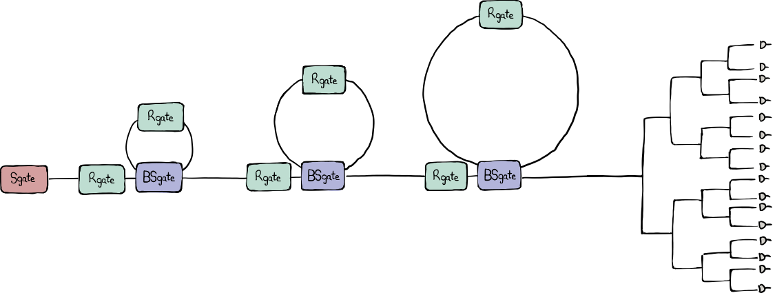
This advanced tutorial will direct more focus on these additional details and help us get a more comprehensive understanding of Borealis and its gate arguments.

Loading the device specification

We start off by importing Strawberry Fields and NumPy, and loading the Borealis device object which contains relevant and up-to-date information about the hardware.

import strawberryfields as sf
import numpy as np

eng = sf.RemoteEngine("borealis")
device = eng.device

Note

This demo is about remotely submitting jobs to our quantum-advantage device Borealis. Borealis is now deprecated, but you can download a dummy device specification and hardware certificate. Load these files and use them to create a device object like what is shown below. This object will allow you to go through most steps of this tutorial, although you won’t be able to run anything on the Borealis hardware device, nor receive any samples.

import json

device_spec = json.load(open("borealis_device_spec.json"))
device_cert = json.load(open("borealis_device_certificate.json"))
device = sf.Device(spec=device_spec, cert=device_cert)

Defining a GBS circuit

As in the beginner’s tutorial, here we will define a GBS circuit similar to the one in the beginner’s tutorial which we can later submit to the hardware and/or to local simulations. This time, we want to define the circuit and all of the gate parameters manually, relying less on the handy convenience functions that we used in the beginner’s tutorial.

In the beginner’s tutorial matching the squeezing values to the closest one supported by the hardware was done behind the scenes. Here, we will instead do it manually by using one of the allowed squeezing values from the device certificate and broadcasting it over a list that is as long as the number of modes that we wish to use.

modes = 216

r0 = device.certificate["squeezing_parameters_mean"]["high"]
r = [r0] * modes

Next, we will define our GBS circuit by randomizing the phase-gate and beamsplitter arguments, very much like we did in the beginner’s tutorial. We will also have to make sure that the loops are completely filled with computational modes at the beginning of the circuit by opening up the loops in the initial time bins by setting them to \(T=1\) (\(\alpha=0\)).

min_phi, max_phi = -np.pi / 2, np.pi / 2
min_T, max_T = 0.4, 0.6

# rotation-gate parameters
phi_0 = np.random.uniform(low=min_phi, high=max_phi, size=modes).tolist()
phi_1 = np.random.uniform(low=min_phi, high=max_phi, size=modes).tolist()
phi_2 = np.random.uniform(low=min_phi, high=max_phi, size=modes).tolist()

# beamsplitter parameters
T_0 = np.random.uniform(low=min_T, high=max_T, size=modes)
T_1 = np.random.uniform(low=min_T, high=max_T, size=modes)
T_2 = np.random.uniform(low=min_T, high=max_T, size=modes)
alpha_0 = np.arccos(np.sqrt(T_0)).tolist()
alpha_1 = np.arccos(np.sqrt(T_1)).tolist()
alpha_2 = np.arccos(np.sqrt(T_2)).tolist()

# the travel time per delay line in time bins
delay_0, delay_1, delay_2 = 1, 6, 36

# set the first beamsplitter arguments to `T=1` (`alpha=0`) to fill the
# loops with pulses
alpha_0[:delay_0] = [0.0] * delay_0
alpha_1[:delay_1] = [0.0] * delay_1
alpha_2[:delay_2] = [0.0] * delay_2

Here comes a tricky part. Although these gate sequences are of length 216 (the number of squeezed-light modes in our GBS instance) the actual time-domain program needs to be longer than that. Why is that the case?

We just imposed that the first computational mode is fully coupled into the first loop. This means that it will arrive at the second loop after exactly one time bin (i.e. one roundtrip in the first delay line). We also imposed that the first mode should be completely coupled into the second loop, which means it will arrive at the third loop no earlier than 7 time bins after the program has started (1 + 6 time bins delay). Therefore, the gates associated to the second and third loop need some idle time bins, awaiting the first computational mode.

To do this, we need to append 0-valued parameters (i.e. full transmission) to the gates in the first two loops. This will make sure that the non-trivial random gates are applied to the computational modes exclusively.

# second loop needs to await the first mode for 1 time bin (delay_0 = 1)
phi_1 = [0] * delay_0 + phi_1
alpha_1 = [0] * delay_0 + alpha_1

# second loop needs to await the first mode for 7 time bins (delay_0 + delay_1 = 1 + 6)
phi_2 = [0] * (delay_0 + delay_1) + phi_2
alpha_2 = [0] * (delay_0 + delay_1) + alpha_2

Toward the end of the time-domain circuit, we need to make sure that all computational modes in the loops are entirely coupled out again, avoiding interfering with the vacuum modes that will follow the pulse train of 216 squeezed-light modes. This means that we need to set the beamsplitters to full transmission again, and, since all gate sequences should have the same length, the gates of the first and second loops need to remain idle until the very last computational mode has exited the third loop.

This requires us to add 0-valued parameters corresponding to the number of modes required to exit through the current and all following loops; i.e., 43 (1 + 6 + 36) for the first loop, 42 (6 + 36) for the second loop, and 36 for the third loop.

# empty first loop (delay_0) and await the emptying of second and third loop
# (delay_1 + delay_2)
r += [0] * (delay_0 + delay_1 + delay_2)
phi_0 += [0] * (delay_0 + delay_1 + delay_2)
alpha_0 += [0] * (delay_0 + delay_1 + delay_2)

# empty second loop (delay_1) and await the emptying of third loop (delay_2)
phi_1 += [0] * (delay_1 + delay_2)
alpha_1 += [0] * (delay_1 + delay_2)

# empty third loop
phi_2 += [0] * delay_2
alpha_2 += [0] * delay_2

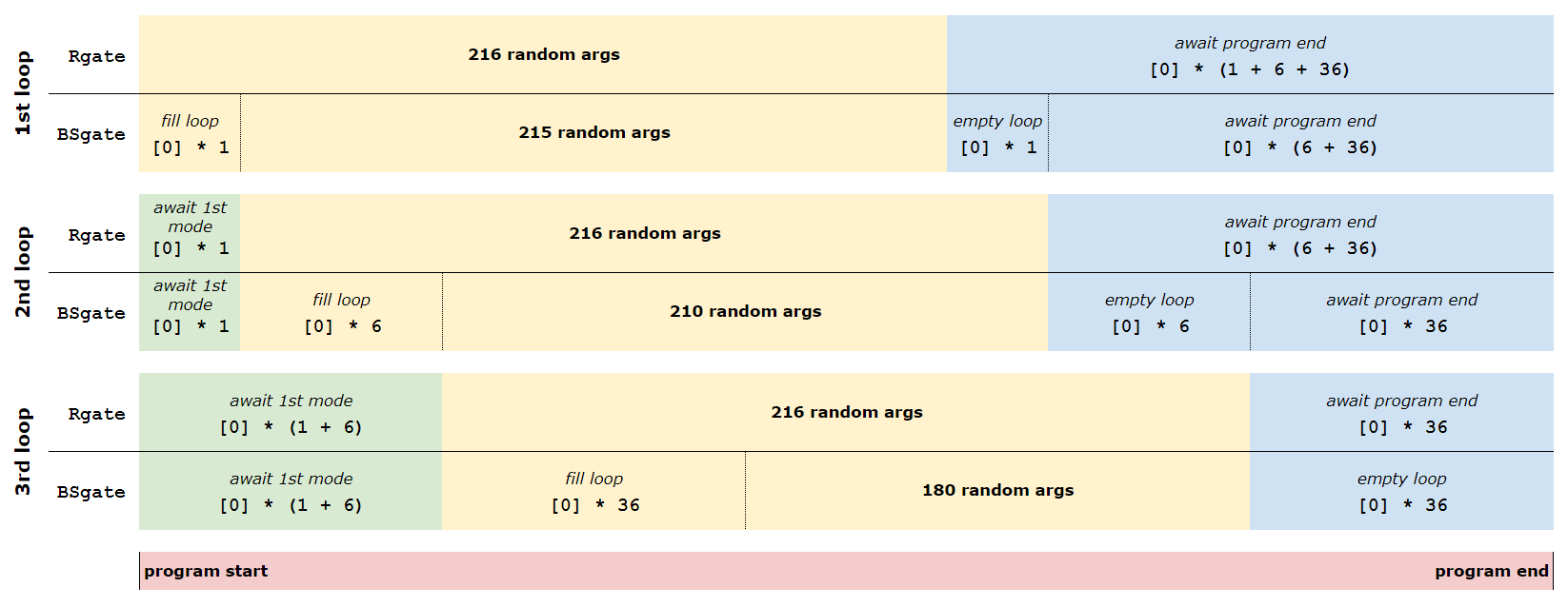
Unfortunately, all of this padding with idle time bins before and after the random gates is necessary to avoid interfering computational modes with vacuum modes. This simply reflects the reality that we need a total unitary that fits the size of the total input state: 216 computational modes and 43 vacuum modes (1, 6, 36 of them in the first, second, and third loop, respectively). Our total unitary thus needs to be of size 259 \(\times\) 259.

The image below provides an overview of the necessary vacuum mode padding for all the three loops, where each row corresponds to a gate parameter array with length 259.

The reward for taking all of these precautions is that the unitary that we desire to implement is now a block matrix within the total unitary, acting on the 216 computational modes exclusively. Moreover, the length of the argument lists submitted to the seven quantum gates is now exactly 259, matching the size of the total unitary. Let’s collect all of the gate sequences in a single nested list that we can submit to the TDMProgram. The list, aptly named gate_args_list, contains all gate parameters in the order in which the corresponding gates will be applied.

gate_args_list = [r, phi_0, alpha_0, phi_1, alpha_1, phi_2, alpha_2]

[len(gate_args) for gate_args in (gate_args_list)]

Out:

[259, 259, 259, 259, 259, 259, 259]

As mentioned in the beginner’s tutorial, each loop applies a static phase rotation to the modes passing through it. Currently, this phase rotation cannot be programmed. All we can do is to measure this phase and take it into account whenever we run a program on the hardware. This is why the three loop offsets "loop_phases" are part of the device certificate. Even though we have no direct control over them, we need to deal with them in order to obtain a correct representation of the circuit that is applied. This can be done in two different ways:

• We include these offsets explicitly into our TDMProgram. In this case, no hidden compensation takes place and the modulators apply the exact phases defined by the user.

• We can stay agnostic about the static offsets and use our phase modulators to actively compensate for them in the background. This is done automatically when the loop offsets are not found in the TDMProgram during compilation. In this case, the Strawberry Fields compiler will absorb the three roundtrip phases into the instructions for the phase modulators such that they effectively apply the user-defined phase-gate arguments. There is a caveat to this approach though, since ~50% of all the loop offsets cannot be compensated for due to the limited range of our phase modulators. In these cases, those phases are shifted by pi.

While in the beginner’s tutorial we went for the second option, we will go with the first option this time. In other words, we will acknowledge the roundtrip phases as part of our circuit and will explicitly add them to our time-domain program. In order to do so, let’s first obtain them from the certificate.

# the intrinsic roundtrip phase of each delay line
phis_loop = device.certificate["loop_phases"]

Executing the circuit

Submit to hardware

From here on, we can proceed very much like we did in the beginner’s tutorial. Only this time, our TDMProgram explicitly includes rotation-gates with the loop-roundtrip phase shifts applied. The results retrieved from running this program on the Borealis device will essentially be the same (albeit with differently randomized parameters) as with the program we ran in the beginner’s tutorial, except for the lack of automatic cropping, which we will do manually instead.

from strawberryfields.tdm import get_mode_indices
from strawberryfields.ops import Sgate, Rgate, BSgate, MeasureFock

delays = [1, 6, 36]
vac_modes = sum(delays)
n, N = get_mode_indices(delays)

prog = sf.TDMProgram(N)
with prog.context(*gate_args_list) as (p, q):
    Sgate(p[0]) | q[n[0]]

    for i in range(len(delays)):
        Rgate(p[2 * i + 1]) | q[n[i]]
        BSgate(p[2 * i + 2], np.pi / 2) | (q[n[i + 1]], q[n[i]])
        Rgate(phis_loop[i]) | q[n[i]]

    MeasureFock() | q[0]

shots = 250_000

eng = sf.RemoteEngine("borealis")
results = eng.run(prog, shots=shots)

Running the circuit remotely on Borealis will return a Result object, which contains the samples that are obtained by the hardware. The samples returned by any TDMProgram are of shape (shots, spatial_modes, temporal_modes), so in our case whe should get a three-dimensional array with shape (shots, 1, 259).

Since the first 43 modes that arrived at the detectors are vacuum modes that live inside the loops before the program starts, we can crop the samples array and focus on the 216 computational modes. Recall from the beginner’s tutorial that this can also be achieved by passing the crop=True flag to the eng.run() call above.

samples = results.samples[..., 43:]

Submit to realistic simulation

Now, let us switch to a local simulation. In order to make it more realistic, we need to take optical loss into account. In the beginner’s tutorial, realistic loss was added automatically by the compiler in the backend. Here, we instead want to insert the various loss components manually into our circuit. The daily calibration routine that runs on Borealis decomposes the total loss suffered by our pulses into three categories:

• eta_glob: The total loss experienced by the different modes depends on which loops they have travelled through and in which detector they ended up. So it will be highly inhomogeneous within the 216 computational modes. eta_glob, on the other hand, describes their common efficiency. It is experienced by a mode that bypasses all three loops and ends up in our most efficient detector. In other words 1 - eta_glob is the minimal loss that every mode will suffer. On top of that, most modes will suffer additional losses imposed by the loops and a less efficient detector.

• eta_loop: Each loop will add an additional loss to each mode that passes through it. eta_loop is a list containing the respective efficiencies of the three loops.

• eta_ch_rel: In the experiment, two consecutive pulses are only 167 ns apart, which exceeds the rate that one single photon-number resolving (PNR) detector can presently handle. So although our batches of 216 squeezed-light modes travel towards the detection module in one single fibre, they need to be demultiplexed into 16 spatial modes, each one of them probed by its own PNR detector. You can find a schematic of our demultiplexing-and-detection module illustrated in the top figure of this tutorial.

We have 16 PNRs operating at 6/16 MHz. The demultiplexing pattern is repetitive, meaning that detector \(i\) will detect all temporal modes whose index satisfies \(i + 16n\), where \(n\) is an integer. Since the 16 spatial modes and their respective detectors do not share the exact same efficiency, eta_ch_rel keeps track of the loss suffered by each one of our modes individually.

All of these loss components can be obtained from the device object.

eta_glob = device.certificate["common_efficiency"]
etas_loop = device.certificate["loop_efficiencies"]
etas_ch_rel = device.certificate["relative_channel_efficiencies"]

Note that the detector-channel efficiencies are cyclic, so mode i sees the same efficiency as mode i + 16, thus necessitating us to repeat the 16 efficiency values for the length of the program. We will also add the channel efficiencies to our list of gate arguments that we submit to the TDMProgram. This is because the relative detection efficiency experienced by the modes needs to be updated at each time bin and is therefore a dynamic TDM gate, very much like the phase modulators and beamsplitters.

prog_length = len(gate_args_list[0])
reps = int(np.ceil(prog_length / 16))
etas_ch_rel = np.tile(etas_ch_rel, reps)[:prog_length]
etas_ch_rel = etas_ch_rel.tolist()

gate_args_list += [etas_ch_rel]

With that, we are now able to redefine the circuit that we submitted to Borealis for simulations under realistic losses.

from strawberryfields.ops import LossChannel

prog_sim = sf.TDMProgram(N)
with prog_sim.context(*gate_args_list) as (p, q):
    Sgate(p[0]) | q[n[0]]
    LossChannel(eta_glob) | q[n[0]]

    for i in range(len(delays)):
        Rgate(p[2 * i + 1]) | q[n[i]]
        BSgate(p[2 * i + 2], np.pi / 2) | (q[n[i + 1]], q[n[i]])
        Rgate(phis_loop[i]) | q[n[i]]
        LossChannel(etas_loop[i]) | q[n[i]]

    LossChannel(p[7]) | q[0]
    MeasureFock() | q[0]

As we have now inserted loss explicitly to the circuit, we can skip any Borealis-specific compiling steps and submit our program directly to the Gaussian backend.

eng_sim = sf.Engine(backend="gaussian")
results_sim = eng_sim.run(prog_sim, shots=None, space_unroll=True)

The covariance matrix returned by results_sim.state.cov() describes our 216 computational modes as well as the 43 vacuum modes that were stored in the loops before executing the program. In the beginner’s tutorial, we made sure that only the computational modes are considered in the covariance matrix by adding crop=True to the run() method. We could have done the same thing here, but instead let’s crop out the vacuum modes manually using the package The Walrus.

from thewalrus.quantum import reduced_gaussian

# total covariance matrix and mean vector describe 259 modes
cov_tot = results_sim.state.cov()
mu_tot = np.zeros(len(cov_tot))

# cropped covariance matrix and mean vector describe 216 modes
mu, cov = reduced_gaussian(mu_tot, cov_tot, range(vac_modes, prog_length))

From here you can use the methods described in the beginner’s tutorial to compare your experimental results to the ones obtained by the simulation.

Note that in the above eng_sim.run() call we added the flag space_unroll=True. This feature was already used and very briefly explained in the beginner’s tutorial. Let’s go into more details here. The circuit above will be rolled-up, using symbolic placeholder variables for the gate parameters. The circuit must be unrolled with each mode only being measured once, a process we call space-unrolling.

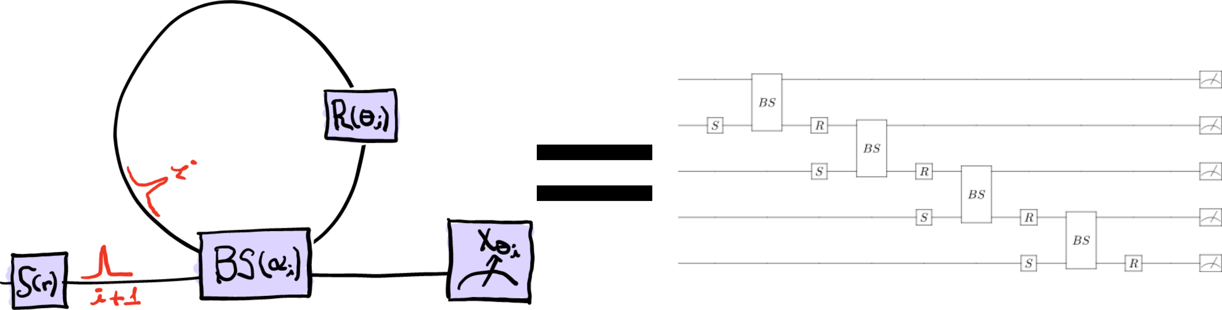
Space-unrolling might seem slightly confusing, but there is a straight-forward way to understand it. Instead of having several modes going through the same path, we interpret the TDM loop interactions as spatially separate. This way, each measurement is made on a different spatial mode, as can be seen in the right-hand side of the image below.

The left-hand side depicts how an actual single loop TDM circuit would work, while the right-hand side is how Strawberry Fields simulates it. Since each mode can only be measured once (i.e., modes cannot be reused when using Fock measurements, opposite to the Entanglement Synthesizer , which uses homodyne measurements), the circuit needs to be unrolled. To get an understanding for how this space-unrolling works, try to follow the interactions happening in the left-hand side single-loop setup, and try to spot them in the right-hand side circuit diagram. They are equal in practice!

Calculating the transfer matrix

The circuit above can be described as a combination of initial state preparation and an interferometer over the 216 modes used in the circuit. This interferometer setup can be described by a so-called transfer matrix. It describes the quantum circuit applied to any initial state. In the absence of loss, the transfer matrix is equivalent to the unitary. By having access to the tranfer matrix, it’s possible to recreate the same circuit using different initial states. Instead of starting with a squeezed state, as we did above, we could, for example, apply the transfer matrix to a coherent state or GKP states.

There is a way to quickly calculate the transfer matrix of a circuit — as long as it only contains beamsplitters, rotation gates and loss channels — without having to execute it. This is done by using the “passive” compiler to compile the circuit into a single transfer gate. Thus, we remove the squeezing from the circuit and simply compile the program using the “passive” compiler, extracting the parameter from the resulting PassiveChannel.

prog_passive = sf.TDMProgram(N)

with prog_passive.context(*gate_args_list, etas_ch_rel) as (p, q):
    LossChannel(eta_glob) | q[n[0]]

    for i in range(len(delays)):
        Rgate(p[2 * i + 1]) | q[n[i]]
        BSgate(p[2 * i + 2], np.pi / 2) | (q[n[i + 1]], q[n[i]])
        Rgate(phis_loop[i]) | q[n[i]]
        LossChannel(etas_loop[i]) | q[n[i]]

    LossChannel(p[7]) | q[0]

prog_passive.space_unroll()

prog_passive = prog_passive.compile(compiler="passive")

Keep in mind that the circuit now only consists of a single PassiveChannel, which has a single matrix parameter. This parameter is the circuit’s transfer matrix. The transfer matrix then allows us to experiment using the same setup, but with different state preparations.

transfer_matrix_tot = prog_passive.circuit[0].op.p[0]

# crop out the vacuum modes
transfer_matrix = transfer_matrix_tot[vac_modes:prog_length, vac_modes:prog_length]

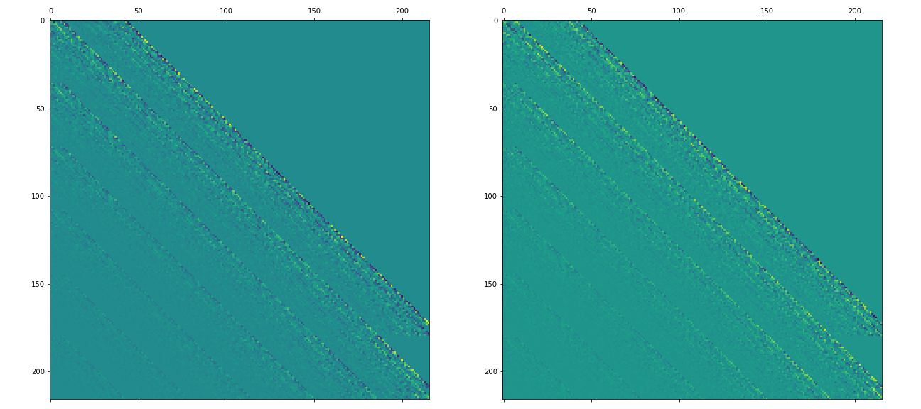
A matrix plot will give us a good intuition on the connectivity of our temporal modes.

import matplotlib.pyplot as plt

fig, ax = plt.subplots(1, 2, figsize=(18, 8))
ax[0].matshow(transfer_matrix.real)
ax[1].matshow(transfer_matrix.imag)
plt.show()

Conclusion

This tutorial covered how to submit jobs to our temporal-division multiplexing device, Borealis. It’s rather exciting to be able to demonstrate the concept of quantum computational advantage by examples running on actual hardware. As you now have seen, there are quite a few details to keep track of, but as long as the circuit follows the correct layout and the parameters are correctly declared, anyone with Xanadu cloud access can submit jobs to be excecuted on the Borealis hardware, and get back samples that would be difficult, if not outright impossible, to retrieve using a local simulator.

We hope that you’ve enjoyed this demonstration, and that you’re as excited as we are about the possibilities. If you wish to dig deeper into the science behind all of this, we recommend that you read our paper [1].

References

1(1,2)

Madsen, L.S., Laudenbach, F., Askarani, M.F. et al. “Quantum computational advantage with a programmable photonic processor”, Nature 606, 75-81, 2022.

About the authors

Theodor Isacsson

Theodor Isacsson is a quantum software developer at Xanadu. He works on the photonics software stack, leading the efforts to expand and maintain packages such as Strawberry Fields and The Walrus.

Fabian Laudenbach

Fabian Laudenbach is an experimental physicist at Xanadu. He is one of the lead authors of the publication showcasing quantum computational advantage with Borealis.

demos/tutorial_borealis_advanced

 

Download Python script

 

Download Notebook