Operating Borealis — Beginner

   Borealis will only be available to the public until June 2, 2023.
   Public access to this device will not be available after this date.

Authors: Fabian Laudenbach and Theodor Isacsson

Note

If you’re in a hurry, check out our Borealis Quickstart.

The demonstration of quantum computational advantage (i.e., the ability of a quantum processor to accomplish a task exponentially faster than any super computer could) is considered an important milestone towards useful quantum computers. One task that is proven to be computationally hard is sampling the photon numbers of multimode squeezed states that have travelled through a non-trivial interferometer — a problem which is referred to as Gaussian Boson Sampling (GBS). In our publication in Nature [1], we showcase a programmable loop interferometer that can successfully sample GBS instances orders of magnitudes faster than any known classical algorithm could using exact methods. The experiment is based on temporal-division multiplexing (TDM) — also known as time-domain multiplexing — which allows for a comparatively simple experimental setup in which the number of optical parts and devices is independent from the number of optical modes. A single squeezed-light source emits batches of 216 time-ordered squeezed-light pulses. These pulses interfere with one another with the help of optical delay loops (acting as memory buffers), programmable beamsplitters, and phase shifters. A simple schematic of the setup can be seen below.

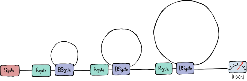
The architecture of our GBS machine – which we call Borealis – is layed out as follows. A squeezed-light source injects pulse trains of 216 modes, temporally spaced by \(\tau = 167~\text{ns}\), into the interferometer which consists of three delay loops that are individually characterized by the roundtrip time it takes a mode to travel trough it. The first, second, and third delay loops have a roundtrip time of \(1 \tau\), \(6 \tau\), and \(36 \tau\), respectively. Each loop is associated with two programmable Gaussian gates; a rotation gate right before the loop and a variable beamsplitter that interferes modes approaching the loop with modes coming from within the loop.

In this tutorial, we will use the TDMProgram class to discuss how a GBS circuit can be programmed on Borealis. This class allows us to define and run time-multiplexed photonic circuits in a very efficient way, even if these circuits include large numbers of modes. For more background on the TDMProgram, please refer to the beginner and advanced tutorials on time-domain photonic circuits.

After defining our GBS circuit, we can either submit the program to the hardware, run a simulation or do both.

Note

This demo is about remotely submitting jobs to our quantum-advantage device Borealis. Borealis is now deprecated, but you can download a dummy device specification and hardware certificate. Load these files and use them to create a device object like what is shown below. This object will allow you to go through most steps of this tutorial, although you won’t be able to run anything on the Borealis hardware device, nor receive any samples.

import json

device_spec = json.load(open("device_specification.json"))
device_cert = json.load(open("device_certificate.json"))
device = sf.Device(spec=device_spec, cert=device_cert)

Loading the device specification

To start off, we import Strawberry Fields along with NumPy, which we will need later on. We then need to load the device object which contains relevant and up-to-date information about Borealis. It includes two dictionaries: the device specification (Borealis uptime, allowed circuit layout, allowed gate parameters) and the device certificate (most recent calibration results).

If you have an API key, you can retrieve the device from the platform upon connecting to Borealis by calling the device property on the RemoteEngine object.

import strawberryfields as sf
import numpy as np

eng = sf.RemoteEngine("borealis")
device = eng.device

The device allows us to make your TDM circuit compatible with our hardware. This is why it is passed to some of the functions defined below. In particular, these functions need to access the latest calibration results which you can view yourself in the device certificate.

device.certificate

Out:

{'target': 'borealis',
 'finished_at': '2022-02-03T15:00:59.641616+00:00',
 'loop_phases': [0.478, 1.337, 0.112],
 'schmidt_number': 1.333,
 'common_efficiency': 0.551,
 'loop_efficiencies': [0.941, 0.914, 0.876],
 'squeezing_parameters_mean': {'low': 0.712, 'high': 1.019, 'medium': 1.212},
 'relative_channel_efficiencies': [0.976,
 0.934,
 0.967,
 1,
 0.921,
 0.853,
 0.919,
 0.939,
 0.877,
 0.942,
 0.919,
 0.987,
 0.953,
 0.852,
 0.952,
 0.945]}

Defining a GBS circuit

A time-domain program is defined by the sequences of arguments each quantum gate applies at each time bin, i.e., on each temporal mode, within the duration of the program. As Borealis is an interferometer with a total of seven Gaussian gates (one squeezer, three rotation gates, and three tunable beamsplitters), we require seven lists of arguments:

• r: sequence of squeezing values

• phi_0, phi_1, phi_2: sequences of arguments applied by the rotation gates

• alpha_0, alpha_1, alpha_2: sequences of arguments applied by the beamsplitters

Fast track

If you do not want to be bothered with defining the gate arguments yourself and just want to run and analyze some GBS instance, simply call the borealis_gbs helper function and proceed to the Executing the circuit section below. The gate_args_list summarizes all the necessary information for Strawberry Fields and our hardware to implement your circuit. In particular, it contains the arguments to be applied by our seven Gaussian gates at each time bin. Your circuit will be roughly equivalent to the ones presented in our publication [1]. All you need to do is to specify the number of modes (up to 288) and a squeezing level ("low", “medium”, or “high”).

We also need to import two other helper functions, which will be explained and used later.

from strawberryfields.tdm import borealis_gbs, full_compile, get_mode_indices

gate_args_list = borealis_gbs(device, modes=216, squeezing="high")

Out:

2022-04-05 10:45:17,350 - WARNING - 136/259 arguments of phase gate 1 have been shifted by pi in order to be compatible with the phase modulators.
2022-04-05 10:45:17,352 - WARNING - 143/259 arguments of phase gate 2 have been shifted by pi in order to be compatible with the phase modulators.

Define your gates manually (optional)

If you want to be more in control of what your circuit should look like, we invite you to follow through with the following couple of steps. Let’s begin by defining the squeezing values, for instance, by creating a list with the same number of parameters as the number of modes in the program.

modes = 216

# squeezing-gate parameters
r = [1.234] * modes

The squeezing values you define will later be matched to the closest one supported by our hardware. You can always view the supported values by calling device.certificate["squeezing_parameters_mean"]. In case you are unsure about what squeezing value to apply, we also support string values instead of numeric lists. You can set r to "zero", "low", "medium", or "high" to access one of the pre-calibrated squeezing levels which will then be applied to all pulses in your program.

For our GBS job, we draw the phase-gate arguments and beamsplitter transmission values from a uniform random distribution. The beamsplitter intensity transmission can be set anywhere between 0 and 1, but in order to obtain a denser adjacency matrix (i.e. a better spread of entanglement throughout the modes) we limit the range to \(T \in [0.4, 0.6]\). Given some intensity transmission \(T\), the argument passed to our beamsplitter will then be \(\alpha=\text{arccos}(\sqrt{T})\). Considering this conversion, we can define our random sequences.

min_phi, max_phi = 0, 2 * np.pi
min_T, max_T = 0.4, 0.6

# rotation-gate parameters
phi_0 = np.random.uniform(low=min_phi, high=max_phi, size=modes)
phi_1 = np.random.uniform(low=min_phi, high=max_phi, size=modes)
phi_2 = np.random.uniform(low=min_phi, high=max_phi, size=modes)

# beamsplitter parameters
T_0 = np.random.uniform(low=min_T, high=max_T, size=modes)
T_1 = np.random.uniform(low=min_T, high=max_T, size=modes)
T_2 = np.random.uniform(low=min_T, high=max_T, size=modes)
alpha_0 = np.arccos(np.sqrt(T_0))
alpha_1 = np.arccos(np.sqrt(T_1))
alpha_2 = np.arccos(np.sqrt(T_2))

Now, we want to set the first arguments of each loop to \(T=1\) (\(\alpha=0\)). This will couple an incoming pulse entirely into the loop, and a vacuum mode that was inside the loop will be coupled out — no interference between the two will occur. For each loop this needs to be repeated until the respective delay line is completely emptied from vacuum modes and filled with computational modes (i.e. optical pulses).

# the travel time per delay line in time bins
delay_0, delay_1, delay_2 = 1, 6, 36

# set the first beamsplitter arguments to 'T=1' ('alpha=0') to fill the
# loops with pulses
alpha_0[:delay_0] = 0.0
alpha_1[:delay_1] = 0.0
alpha_2[:delay_2] = 0.0

For convenience, let’s collect the gate arguments in a dictionary. This can also be done with the helper function to_args_dict, but we will show the dictionary creation manually for clarity.

gate_args = {
    "Sgate": r,
    "loops": {
        0: {"Rgate": phi_0.tolist(), "BSgate": alpha_0.tolist()},
        1: {"Rgate": phi_1.tolist(), "BSgate": alpha_1.tolist()},
        2: {"Rgate": phi_2.tolist(), "BSgate": alpha_2.tolist()},
    },
}

Before we can submit these gates to Strawberry Fields, we need to make some adjustments to the lists in order to account for the peculiarities of our hardware and TDM circuits in general:

• Squeezing level: Only a discrete set of squeezing parameters is properly calibrated. These are the values that the hardware is able to apply. The squeezing values in your r list need to be matched to the closest value that is supported by the hardware.

• Mode delay: Note that the gate sequences you have defined for the respective loops do not necessarily start at the same time. It all depends on how long the arrival of the first pulse at a respective loop (and its rotation and beamsplitter gate) has been delayed by previous loops. Therefore, the time that each gate sequence starts has to be delayed accordingly.

• Emptying the delay loops: When your time-domain circuit is over, there might still be some pulses travelling in the fibre loops. The variable beamsplitters must be set such that these modes can exit the loops and travel to the detector module.

• Phase corrections: On top of applying the phase-gate arguments that you ask for, our phase modulators need to compensate for other, static, non-programmable phase offsets in the setup. In some cases, the offset-corrected phase falls beyond range of the modulators. So we want to make sure that all the phase-gate arguments submitted to the TDMProgram can actually be implemented in the presence of the non-programmable phase offsets.

These compilation steps can be carried out individually (manually, or by calling the respective Strawberry Fields helper functions) as described in the advanced tutorial. However, we can conveniently call the full_compile function which takes care of all these steps at once.

gate_args_list = full_compile(gate_args, device)

Out:

2022-04-05 10:47:24,388 - WARNING - Submitted squeezing values have been matched to the closest median value supported by hardware: ['0.000', '0.150', '0.350', '0.550'].
2022-04-05 10:47:24,391 - WARNING - 129/259 arguments of phase gate 1 have been shifted by pi in order to be compatible with the phase modulators.
2022-04-05 10:47:24,391 - WARNING - 143/259 arguments of phase gate 2 have been shifted by pi in order to be compatible with the phase modulators.

Note

As mentioned above, we sometimes need to delay the beginning of the gate sequences depending on the delay applied by previous loop(s) at the arrival of the first pulse so that they can start right on time. Also, we want a program to end with open loops in order to give all modes the opportunity to exit the delay loops and travel to the detectors. Both of these goals are achieved by adding particular amounts of zeros to the beginning and end of the respective gate lists. This is why after calling full_compile(), your gate lists have grown, which you can easily verify yourself. Visit the advanced tutorial for more details.

Executing the circuit

In order to execute a circuit we need to submit it to a Strawberry Fields TDMProgram. Our first step will be to declare the delays in the loops, i.e. the number of modes that will fit in each loop at the same time. We can then use a helper function called get_mode_indices to get the number of modes that are alive at the same time (concurrent modes) N, which is required for initializing the TDMProgram, and the correct mode indices n for the circuit gates. The parameter n helps us to define the TDMProgram in a really concise way, as you will see below.

delays = [1, 6, 36]
vac_modes = sum(delays)

n, N = get_mode_indices(delays)

Finally, we can construct the circuit. The layout of this circuit is set by the hardware device and cannot be changed. If the wrong gates are used or they are put in the wrong order, the circuit validation will fail.

from strawberryfields.ops import Sgate, Rgate, BSgate, MeasureFock

prog = sf.TDMProgram(N)

with prog.context(*gate_args_list) as (p, q):
    Sgate(p[0]) | q[n[0]]
    for i in range(len(delays)):
        Rgate(p[2 * i + 1]) | q[n[i]]
        BSgate(p[2 * i + 2], np.pi / 2) | (q[n[i + 1]], q[n[i]])
    MeasureFock() | q[0]

Submit to hardware and analyze results

After constructing the circuit, now uniquely defined by the prog object, we can submit it to Borealis by calling and running the RemoteEngine object that we created above. If you do not have an API key, continue on to the Submit to local simulation and compare to hardware results section below.

shots = 250_000
results = eng.run(prog, shots=shots, crop=True)

samples = results.samples

Out:

2022-04-05 10:48:47,057 - INFO - Compiling program for device borealis using compiler borealis.
2022-04-07 10:48:51,999 - INFO - The remote job 36424646-45bc-4de2-a01b-e078766fa78e has been completed.

Note

Depending on how long the first optical pulse is delayed by the respective loops, the circuit will measure a couple of empty modes at the beginning. The crop=True flag will make sure these empty modes are not returned.

Running the circuit remotely on Borealis will return a Result object which contains the samples that are obtained by the machine. The samples returned by any TDMProgram are of shape (shots, spatial modes, temporal modes). So, in our case we should have received samples of shape (shots, 1, 216).

If you followed through with the above steps, you have just run a GBS instance of the same type as demonstrated in our manuscript [1]! This paper also explains how to obtain the estimated runtime required by Fugaku (currently the world’s most powerful classical supercomputer) to simulate the individual GBS samples. You can compute these runtimes for the GBS samples that you just created using the Strawberry Fields utility function gbs_sample_runtime. Note, however, that this analysis is based on the current Fugaku specs (characterized by the LINPACK supercomputer benchmarks) and on the best known algorithm to compute Hafnians. Therefore, this estimation of simulation runtime can be affected in the future by the advent of more powerful computers and/or more efficient algorithms.

from strawberryfields.utils import gbs_sample_runtime

runtimes = np.array([gbs_sample_runtime(sample[0]) for sample in samples])

Let us illustrate the simulation runtimes in a histogram using matplotlib.pyplot.

import matplotlib.pyplot as plt

fs_axlabel = 22
fs_text = 20
fs_ticklabel = 21
fs_legend = 20


def plot_simulation_time(runtimes):
    """Plots a histogram with simulation times.

    Args:
        runtimes (array[float]): the runtimes per GBS sample
    """
    runtimes_log_years = np.log10(runtimes / 365 / 24 / 3600)
    max_exponent = int(max(runtimes_log_years))
    min_exponent = int(min(runtimes_log_years))

    _, ax = plt.subplots(figsize=(18, 8))
    bins = np.arange(min_exponent, max_exponent + 1)
    ax.hist(runtimes_log_years, width=0.8, bins=bins - 0.4)
    ax.set_xlabel(r"simulation time [log$_{10}$ years]", fontsize=fs_axlabel)
    ax.set_ylabel("occurrence", fontsize=fs_axlabel)
    ax.set_yscale("log")
    ax.tick_params(axis="x", labelsize=fs_ticklabel)
    ax.tick_params(axis="y", labelsize=fs_ticklabel)
    ax.set_xticks(bins)

    plt.show()


plot_simulation_time(runtimes)

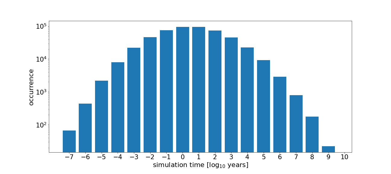
We can also print the median and average simulation time per sample, the simulation time of your brightest sample (the one with the most photons in it), and the time it would take to simulate all the samples you created.

runtime_data = f"""
simulation runtimes [years]
median: {np.median(runtimes) / 365 / 24 / 3600:.1E}
average: {np.mean(runtimes) / 365 / 24 / 3600:.1E}
brightest: {np.max(runtimes) / 365 / 24 / 3600:.1E}
total: {np.sum(runtimes) / 365 / 24 / 3600:.1E}
"""

print(runtime_data)

Out:

simulation runtimes [years]
median: 3.9E+00
average: 2.3E+05
brightest: 2.0E+10
total: 1.1E+11

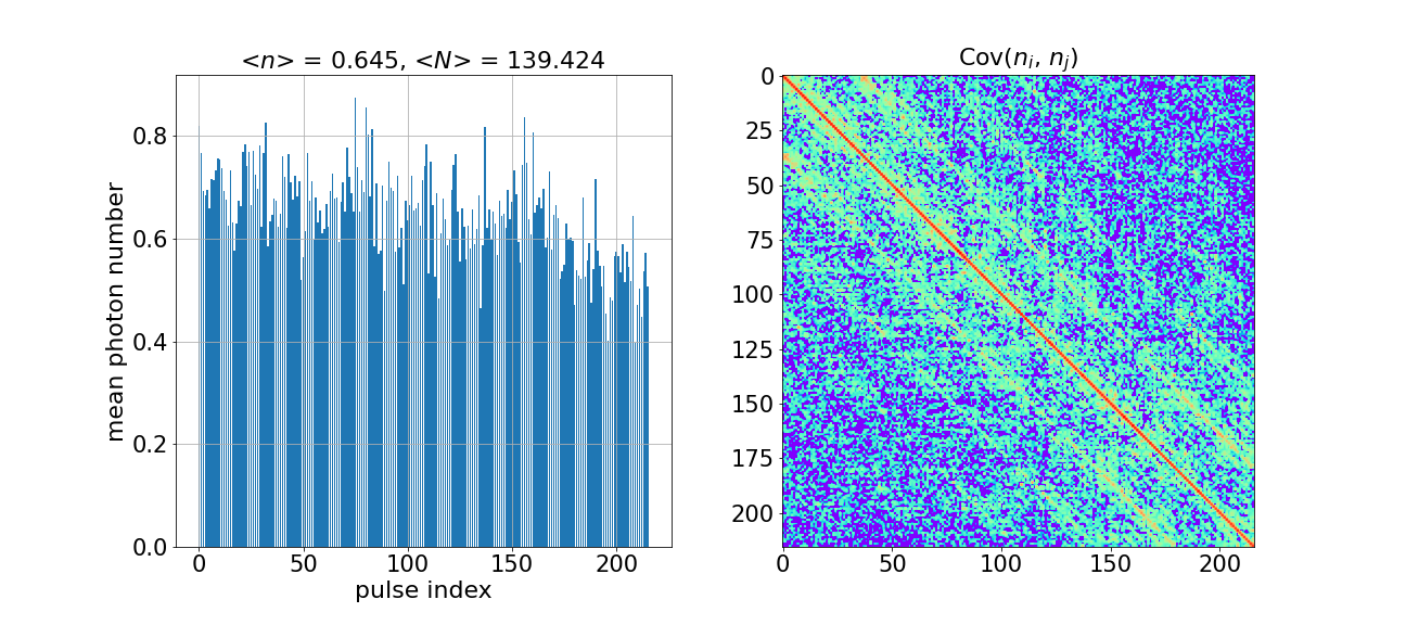
Next, let us look at the statistical moments of our samples. The following two functions will return an array of mean photon numbers for the 216 modes and a \(216 \times 216\) photon-number covariance matrix whose elements are defined by \(\text{Cov}(n_{i}, n_{j}) = E(n_{i} n_{j}) - E(n_{i}) E(n_{j})\).

mean_n = np.mean(samples, axis=(0, 1))
cov_n = np.cov(samples[:, 0, :].T)

Let’s visualize these two results in a figure. This figure can then be used to compare the hardware outcome with local simulations.

import matplotlib.colors


def plot_photon_number_moments(mean_n, cov_n):
    """Plots first and second moment of the photon-number distribution.

    Args:
        mean_n (array[float]): mean photon number per mode
        cov_n (array[int]): photon-number covariance matrix
    """
    _, ax = plt.subplots(1, 2, figsize=(18, 8))

    ax[0].bar(range(len(mean_n)), mean_n, width=0.75, align="center")
    ax[0].set_title(
        rf"<$n$> = {np.mean(mean_n):.3f}, <$N$> = {np.sum(mean_n):.3f}",
        fontsize=fs_axlabel,
    )
    ax[0].set_xlabel("pulse index", fontsize=fs_axlabel)
    ax[0].set_ylabel("mean photon number", fontsize=fs_axlabel)
    ax[0].grid()
    ax[0].tick_params(axis="x", labelsize=fs_ticklabel)
    ax[0].tick_params(axis="y", labelsize=fs_ticklabel)

    ax[1].imshow(
        cov_n,
        norm=matplotlib.colors.SymLogNorm(
            linthresh=10e-6, linscale=1e-4, vmin=0, vmax=2
        ),
        cmap="rainbow",
    )
    ax[1].set_title(r"Cov($n{_i}$, $n{_j}$)", fontsize=fs_axlabel)
    ax[1].tick_params(axis="x", labelsize=fs_ticklabel)
    ax[1].tick_params(axis="y", labelsize=fs_ticklabel)

    plt.show()


plot_photon_number_moments(mean_n, cov_n)

Submit to local simulation and compare to hardware results

Now, let us switch to a local simulation and see how the results compare against the experimental data. By design, Borealis is an experiment that is difficult to sample from classically. What the simulator devices cannot do is return actual samples the same way the remote engine does, at least not in a reasonable amount of time. Setting shots=None in the Engine.run call below makes sure that the local engine doesn’t even attempt to simulate GBS outcomes. Still, even though the engine won’t return samples, running the circuit locally on the Gaussian backend returns a Result object with many other interesting properties.

Loss channels will be added to the program to make the simulation more realistic. To do this, the actual efficiency values obtained in the most recent Borealis calibration run, which are stored in the device certificate, will be used during the compilation process.

We begin by collecting the options that we wish to pass to the compiler prior to running the simulation. To apply realistic loss, instead of using the default backend compiler we need to compile the program using the Borealis compiler. We also need to pass the device along to the engine since it’s required by the Borealis compiler and also contains the relevant efficiency values used when applying the loss.

compile_options = {
    "device": device,
    "realistic_loss": True,
}

Finally, we can run the program on the Gaussian backend, setting the number of shots to None — meaning that no sampling will be attempted — and the crop keyword to True, cropping away the empty modes at the beginning. We also need to tell the engine to space-unroll the circuit before running it. Otherwise, the simulation will only handle the concurrent modes, i.e. the modes that are simultaneously alive at a given time (in our case 44), causing the final state to only contain a subset of all the modes. You can read more about space-unrolling in the advanced tutorial.

To make the code a bit cleaner, we collect all run options in a dictionary which we can unwrap in the run call signature.

run_options = {
    "shots": None,
    "crop": True,
    "space_unroll": True,
}

eng_sim = sf.Engine(backend="gaussian")
results_sim = eng_sim.run(prog, **run_options, compile_options=compile_options)

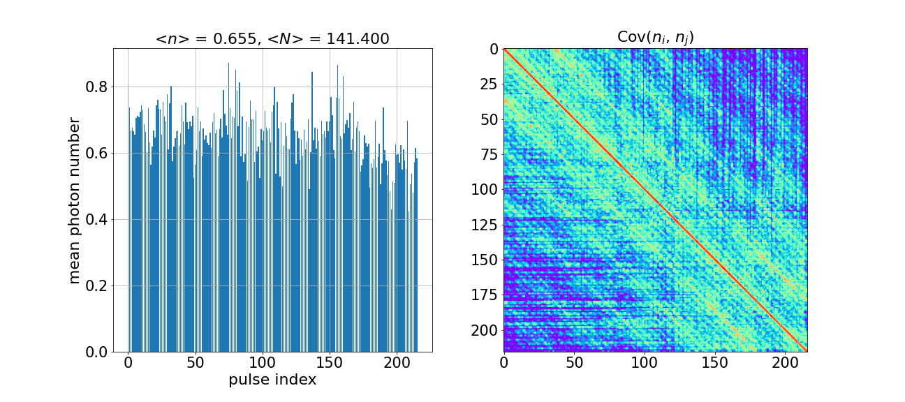
When executing the program on a simulator device, we can extract the covariance matrix by calling the cov() method on the returned state, which is not possible when running on Borealis.

cov = results_sim.state.cov()

The covariance matrix describes the quadrature relations of the individual modes and, in the absence of displacements, contains the full information of the Gaussian state. However, if we want to be able to compare the simulation against experimental data, we would like to obtain the same photon-number statistics as above: the array of mean photon numbers for the 216 modes and a \(216 \times 216\) photon-number covariance matrix. We can use photon_number_mean_vector() and photon_number_covmat(), two functions from Xanadu’s open-source library The Walrus, to obtain these distributions from the quadrature covariance matrix.

from thewalrus.quantum import (
    photon_number_mean_vector,
    photon_number_covmat,
)

mu = np.zeros(len(cov))
mean_n_sim = photon_number_mean_vector(mu, cov)
cov_n_sim = photon_number_covmat(mu, cov)

plot_photon_number_moments(mean_n_sim, cov_n_sim)

If you have submitted the same circuit to both Borealis and the local simulator backend, following the steps above, you should be able to compare the two results. We can also visualize the similarities between the two using scatter plots with the first and second moments of the simulated and experimental photon-number distributions.

def plot_photon_number_moment_comparison(mean_n_exp, mean_n_sim, cov_n_exp, cov_n_sim):
    """Plot first and second moment of the PNR distribution.

    Compare in scatter plots the first and second moments of the photon-number
    distribution resulting from experiment and simulation.

    Args:
        mean_n_exp (array): experimental mean photon number per mode
        mean_n_sim (array): simulated mean photon number per mode
        cov_n_exp (array): experimental photon-number covariance matrix
        cov_n_sim (array): simulated photon-number covariance matrix
    """
    cov_n_exp2 = np.copy(cov_n_exp)
    cov_n_sim2 = np.copy(cov_n_sim)

    # remove the diagonal elements (corresponding to the single-mode variance)
    # which would otherwise be dominant
    cov_n_exp2 -= np.diag(np.diag(cov_n_exp2))
    cov_n_sim2 -= np.diag(np.diag(cov_n_sim2))

    _, ax = plt.subplots(1, 2, figsize=(18, 8))

    min_ = np.min([mean_n_sim, mean_n_exp])
    max_ = np.max([mean_n_sim, mean_n_exp])
    ax[0].scatter(mean_n_sim, mean_n_exp, s=4, alpha=0.50)
    ax[0].plot([min_, max_], [min_, max_], "k--")
    ax[0].set_title("1st moment", fontsize=fs_axlabel)
    ax[0].set_xlabel("simulation", fontsize=fs_axlabel)
    ax[0].set_ylabel("experiment", fontsize=fs_axlabel)
    ax[0].set_xlim([min_, max_])
    ax[0].set_ylim([min_, max_])
    ax[0].set_aspect("equal", adjustable="box")
    ax[0].tick_params(axis="x", labelsize=fs_ticklabel)
    ax[0].tick_params(axis="y", labelsize=fs_ticklabel)
    ax[0].grid()

    min_ = np.min([cov_n_sim2, cov_n_exp2])
    max_ = np.max([cov_n_sim2, cov_n_exp2])
    ax[1].scatter(cov_n_sim2, cov_n_exp2, s=4, alpha=0.50)
    ax[1].plot([min_, max_], [min_, max_], "k--")
    ax[1].set_title("2nd moment", fontsize=fs_axlabel)
    ax[1].set_xlabel("simulation", fontsize=fs_axlabel)
    ax[1].set_ylabel("experiment", fontsize=fs_axlabel)
    ax[1].set_xlim([min_, max_])
    ax[1].set_ylim([min_, max_])
    ax[1].set_aspect("equal", adjustable="box")
    ax[1].tick_params(axis="x", labelsize=fs_ticklabel)
    ax[1].tick_params(axis="y", labelsize=fs_ticklabel)
    ax[1].grid()

    plt.show()


plot_photon_number_moment_comparison(mean_n, mean_n_sim, cov_n, cov_n_sim)

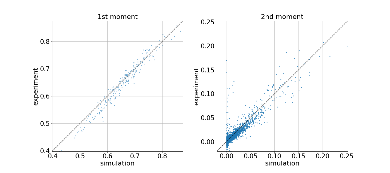
If everything is working as expected, the scatter points should be distributed close to the diagonals. This means that the experiment and simulation are in good agreement with one another.

Conclusion

This tutorial covered how to submit jobs to our temporal-division multiplexing device Borealis. It’s rather exciting to be able to demonstrate the concept of quantum computational advantage by examples running on actual hardware. As you have now seen, there are quite a few details to keep track of. As long as the circuit follows the correct layout and the parameters are correctly declared, anyone with Xanadu cloud access can submit jobs to be executed on Borealis and get back samples that would be difficult, if not outright impossible, to retrieve using a local simulator.

You can find some more examples of how to visualize your data here.

We hope that you’ve enjoyed this demonstration and that you’re as excited as we are about the possibilities. If you wish to dig deeper into the science behind all of this, we recommend that you read our paper [1] and check out our advanced Borealis tutorial.

References

1(1,2,3,4)

Madsen, L.S., Laudenbach, F., Askarani, M.F. et al. “Quantum computational advantage with a programmable photonic processor”, Nature 606, 75-81, 2022.

About the authors

Theodor Isacsson

Theodor Isacsson is a quantum software developer at Xanadu. He works on the photonics software stack, leading the efforts to expand and maintain packages such as Strawberry Fields and The Walrus.

Fabian Laudenbach

Fabian Laudenbach is an experimental physicist at Xanadu. He is one of the lead authors of the publication showcasing quantum computational advantage with Borealis.

demos/tutorial_borealis_beginner

 

Download Python script

 

Download Notebook