Vibronic spectra

Technical details are available in the API documentation: sf.apps.qchem.vibronic

Here we study how GBS can be used to compute vibronic spectra. So let’s start from the beginning: what is a vibronic spectrum? Molecules absorb light at frequencies that depend on the allowed transitions between different electronic states. These electronic transitions can be accompanied by changes in the vibrational energy of the molecules. In this case, the absorption lines that represent the frequencies at which light is more strongly absorbed are referred to as the vibronic spectrum. The term vibronic refers to the simultaneous vibrational and electronic transitions of a molecule upon absorption of light.

It is possible to determine vibronic spectra by running clever and careful spectroscopy experiments. However, this can be slow and expensive, in which case it is valuable to predict vibronic spectra using theoretical calculations. To model molecular vibronic transitions with GBS, we need only a few relevant molecular parameters:

1. \(\Omega\): diagonal matrix whose entries are the square-roots of the frequencies of the normal modes of the electronic initial state.

2. \(\Omega'\): diagonal matrix whose entries are the square-roots of the frequencies of the normal modes of the electronic final state.

3. \(U_\text{D}\): Duschinsky matrix.

4. \(\delta\): displacement vector.

5. \(T\): temperature.

The Duschinsky matrix and displacement vector encode information regarding how vibrational modes are transformed when the molecule changes from the initial to final electronic state. At zero temperature, all initial modes are in the vibrational ground state. At finite temperature, other vibrational states are also populated.

In the GBS algorithm for computing vibronic spectra [1], these chemical parameters are sufficient to determine the configuration of a GBS device. As opposed to other applications that involve only single-mode squeezing and linear interferometry, in vibronic spectra we prepare a Gaussian state using two-mode squeezing, linear interferometry, single-mode squeezing, and displacements.

The function gbs_params() of the vibronic module can be used to obtain the squeezing, interferometer, and displacement parameters from the input chemical parameters listed above. In this page, we study the vibronic spectrum of formic acid 🐜. Its chemical parameters, obtained from [1], can be found in the data module:

from strawberryfields.apps import data, qchem
import numpy as np

formic = data.Formic()
w = formic.w  # ground state frequencies
wp = formic.wp  # excited state frequencies
Ud = formic.Ud  # Duschinsky matrix
delta = formic.delta  # displacement vector
T = 0  # temperature

We can now map this chemical information to GBS parameters using the function gbs_params():

t, U1, r, U2, alpha = qchem.vibronic.gbs_params(w, wp, Ud, delta, T)

Note that since two-mode squeezing operators are involved, if we have \(N\) vibrational modes, the Gaussian state prepared is a \(2N\)-mode Gaussian state and the samples are vectors of length \(2N\). The first \(N\) modes are those of the final electronic state; the remaining \(N\) modes are those of the ground state. From above, \(t\) is a vector of two-mode squeezing parameters, \(U_1\) and \(U_2\) are the interferometer unitaries (we need two interferometers), \(r\) is a vector of single-mode squeezing parameters, and alpha is a vector of displacements.

Photons detected at the output of the GBS device correspond to a specific transition energy. The GBS algorithm for vibronic spectra works because the programmed device provides samples in such a way that the energies that are sampled with high probability are the peaks of the vibronic spectrum. The function energies() can be used to compute the energies for a set of samples. In this case we show the energy of the first five samples:

e = qchem.vibronic.energies(formic, w, wp)
print(np.around(e[:5], 4))  # 4 decimal precision

Out:

[1566.4602 4699.3806 1566.4602 4699.3806 4699.3806]

Once the GBS parameters have been obtained, it is straightforward to run the GBS algorithm: we generate many samples, compute their energies, and make a histogram of the observed energies. The sample() function is tailored for sampling from vibronic spectra. Similarly, the plot module includes a spectrum() function that generates the vibronic spectrum from the GBS samples. Let’s see how this is done for just a few samples:

from strawberryfields.apps import plot

nr_samples = 10

s = qchem.vibronic.sample(t, U1, r, U2, alpha, nr_samples)
e = qchem.vibronic.energies(s, w, wp)
plot.spectrum(e, xmin=-1000, xmax=8000)

The bars in the plot are the histogram of energies. The curve surrounding them is a Lorentzian broadening of the spectrum, which better represents the observations from an actual experiment. Of course, 10 samples are not enough to accurately reconstruct the vibronic spectrum. Let’s instead use the 20,000 pre-generated samples from the data module.

e = qchem.vibronic.energies(formic, w, wp)
plot.spectrum(e, xmin=-1000, xmax=8000)

We can compare this prediction with an actual experimental spectrum, obtained from Fig. 3 in Ref. [1], shown below:

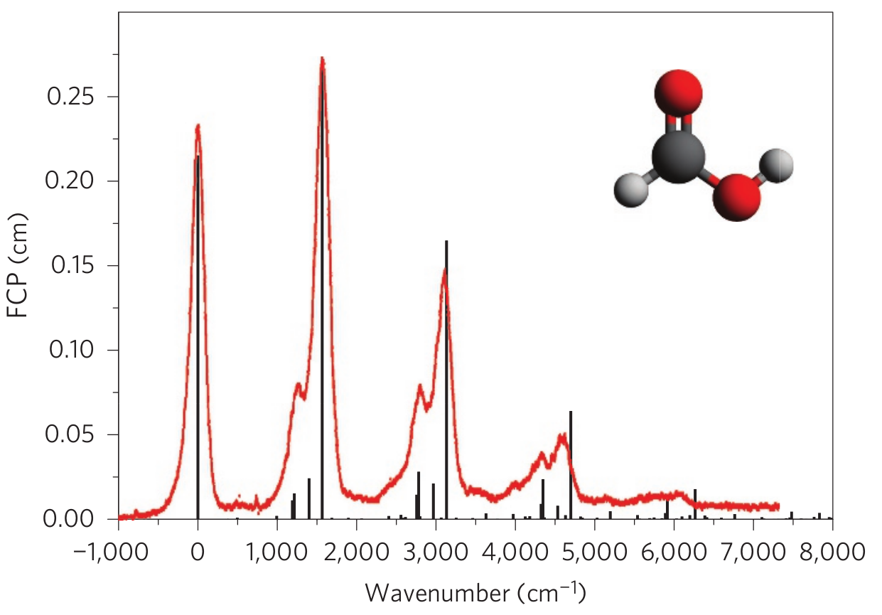
The agreement is remarkable! Formic acid is a small molecule, which means that its vibronic spectrum can be computed using classical computers. However, for larger molecules, this task quickly becomes intractable, for much the same reason that simulating GBS cannot be done efficiently with classical devices. Photonic quantum computing therefore holds the potential to enable new computational capabilities in this area of quantum chemistry ⚛️.

References

1(1,2,3)

Joonsuk Huh, Gian Giacomo Guerreschi, Borja Peropadre, Jarrod R. McClean, and Alán Aspuru-Guzik. Boson sampling for molecular vibronic spectra. Nature Photonics, 9(9):615–620, Aug 2015. URL: http://dx.doi.org/10.1038/nphoton.2015.153, doi:10.1038/nphoton.2015.153.

apps/run_tutorial_vibronic

 

Download Python script

 

Download Notebook