Vibrational dynamics

Technical details are available in the API documentation: sf.apps.qchem.dynamics

Molecules vibrate! In simple cases, like molecular oxygen, atoms can only vibrate along a single axis: O=O –> O===O –> O=O –> O===O. For larger molecules consisting of many atoms, vibrations can become much more complicated and fascinating. A useful tool for understanding vibrations is the concept of normal modes. These are patterns of vibration such that all components of a system move synchronously and with the same frequency, even if they do so in different directions. If a molecule is vibrating in a normal mode, its vibrational dynamics are straightforward: it continues to vibrate in the same pattern.

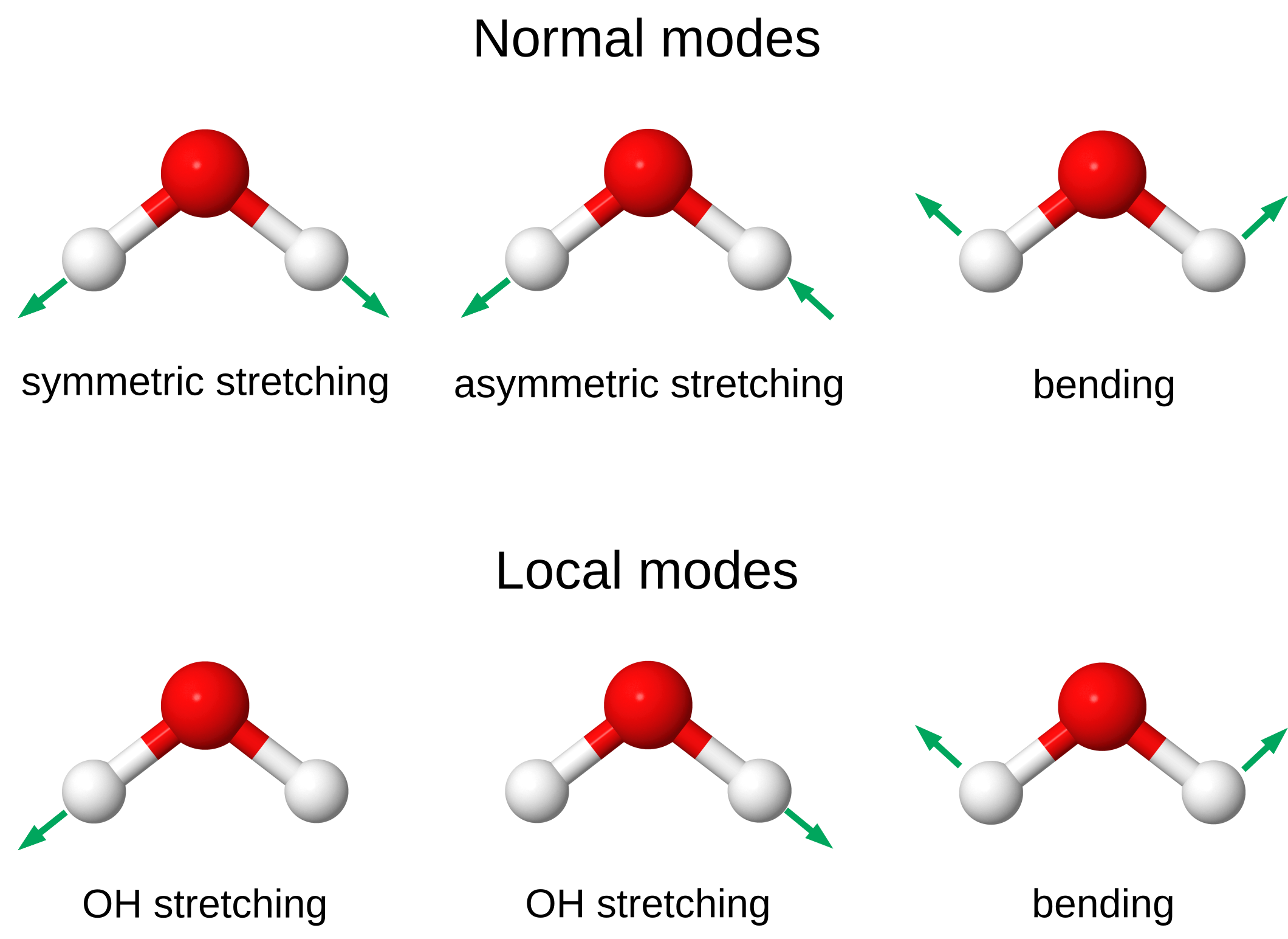
More interesting is the situation where a polyatomic molecule vibrates in a pattern that is not a normal mode, e.g., when the vibration is localized on specific atomic positions or chemical bonds. These patterns are referred to as local modes, and their evolution in time is more challenging to predict and analyze. As an illustration, consider the case of the water molecule shown in the figure below. Water has three vibrational normal modes: the symmetric and asymmetric stretching modes, and a bending mode. These normal modes can be transformed to three local modes: two stretching modes describing the vibrations of the single OH bonds, and a bending mode. Note that the bending mode is already localized.

The dynamics of the vibrational excitations in the normal and local modes of molecules are important to understand the mechanism of chemical reactions and energy transport [1], [2]. For instance, the time-dependent accumulation of vibrational energy in a specific stretching mode can break chemical bonds or change the reactivity of a molecule.

Within the so-called harmonic approximation, normal vibrational modes are orthogonal to each other and excitations in one mode do not lead to excitations in the other modes. Local modes, on the other hand, are not orthogonal and the time evolution of vibrational excitations in local modes is not trivial. Simulation of the dynamics of vibrations excitations in local modes requires solving the time-dependent Schrödinger equation, which is computationally expensive with classical methods.

In this tutorial, we explain how to use Gaussian Boson Sampling (GBS) for simulating the time evolution of vibrational excitations in local modes [1], [2]. Here’s the main idea. First, we exploit a correspondence between vibrational modes in a molecule and optical modes in a photonic quantum computer. In this case, photons in the device represent vibrational quanta. Second, given an initial state of the molecule in the basis of local modes, we transform the system to the basis of normal modes, where time evolution can be described more simply. This local-to-normal transformation is given by a unitary operation which can be implemented with an interferometer. Once time evolution has been performed, we convert back to the local basis and probe the local modes to determine the number of vibrational quanta.

Here’s the algorithm in more detail:

1. Assign each local mode in the molecule to a corresponding optical mode in the GBS device.

2. Prepare an initial state in which some local modes are vibrationally excited.

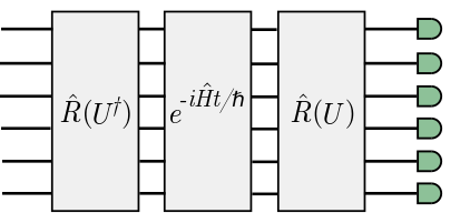
3. Apply the unitary \(U^{\dagger}\) to transform the local modes to the normal basis.

4. Perform time evolution of the quantum state by applying the transformation \(\exp(-i \hat{H} t / \hbar)\). Here \(\hat{H} = \sum_i \hbar \omega_i a_i^\dagger a_i\) defines a Hamiltonian of independent quantum harmonic oscillators, \(\omega_i\) is the vibrational frequency of the \(i\)-th normal mode, \(t\) is time, and \(\hbar\) is Planck’s constant.

5. Apply the unitary \(U\) to transform the normal modes to the local modes.

6. Measure the number of photons in each mode.

The distribution of the photons in the final modes determines the number of vibrational quanta in the local modes. The GBS setup that corresponds to this algorithm is schematically illustrated below.

Vibrational dynamics of water

We are now ready to simulate vibrational quantum dynamics with GBS. In this tutorial, we will focus on one of the most iconic molecules of all time: water 🌊. We first import the modules we need.

import matplotlib.pyplot as plt
import numpy as np
import strawberryfields as sf
from strawberryfields.apps import qchem

We also need the molecular parameters that are used to program the GBS device. These parameters are (i) the normal-to-local unitary \(U\), and (ii) the vibrational frequencies of the normal modes [1]. Following common conventions in quantum chemistry, these frequencies are quoted in units of \(\mbox{cm}^{-1}\). The vibrational normal modes and frequencies can be obtained from electronic structure calculations. The procedure for computing the normal-to-local unitary is explained in [3].

w = sf.apps.data.Water(0).w
U = sf.apps.data.Water(0).U

We now define an engine and initialize our quantum program. We also need to define the number of modes and a cutoff dimension \(D\) which determines the restricted set of number states \(\{|0\rangle , ..., |D − 1\rangle\}\) for each mode [4]. We use Fock states as the initial state in the GBS circuit, which represent states with a fixed number of vibrational quanta.

modes = 3
eng = sf.Engine("fock", backend_options={"cutoff_dim": 5})
prog = sf.Program(modes)

We prepare an initial Fock state in which the second local OH stretching mode is populated with one vibrational quantum, corresponding to a single photon in the GBS device.

input_state = [0, 1, 0]

We define the time (in femtoseconds) and the number of samples to be generated. First we generate 10 samples at t = 70 femtoseconds.

t = 70
n_samples = 10

We use the function TimeEvolution() to evolve the quantum state in time. Given a set of frequencies and a time of evolution \(t\), this function applies a set of rotation gates on the quantum state, which are parameterized according to the transformation \(\exp(-i \hat{H} t / \hbar)\). The normal-to-local transformation unitary is mapped to an interferometer. Note that we apply the transpose first, then convert back without transposing.

# to make samples reproducible
np.random.seed(seed=42)

samples = []

with prog.context as q:
    for i in range(modes):
        sf.ops.Fock(input_state[i]) | q[i]
    sf.ops.Interferometer(U.T) | q
    qchem.dynamics.TimeEvolution(w, t) | q
    sf.ops.Interferometer(U) | q
    sf.ops.MeasureFock() | q

for _ in range(n_samples):
    samples.append(eng.run(prog).samples[0].tolist())

Let’s take a look at the samples.

print(*samples, sep="\n")

Out:

[0, 1, 0]
[1, 0, 0]
[1, 0, 0]
[1, 0, 0]
[0, 1, 0]
[0, 1, 0]
[0, 1, 0]
[1, 0, 0]
[1, 0, 0]
[1, 0, 0]

Now, let’s compute the mean photon numbers in each mode.

print(np.mean(samples, axis=0))

Out:

[0.6 0.4 0. ]

At time 70 femtoseconds, the excitations are also observed in the first local OH stretching mode. We can create a sampling function based on the circuit implemented above and use it to generate samples at any desired time.

def sample(input_state, t, w, U, n_samples):
    modes = len(U)
    samples = []
    eng = sf.Engine("fock", backend_options={"cutoff_dim": 5})
    prog = sf.Program(modes)

    with prog.context as q:
        for i in range(modes):
            sf.ops.Fock(input_state[i]) | q[i]
        sf.ops.Interferometer(U.T) | q
        qchem.dynamics.TimeEvolution(w, t) | q
        sf.ops.Interferometer(U) | q
        sf.ops.MeasureFock() | q

    for _ in range(n_samples):
        samples.append(eng.run(prog).samples[0].tolist())
    return samples

We can repeat the sampling at different times and plot the probability of observing excitations in the local vibrational modes of water as a function of time. Since the sampling process is time-consuming, we import pre-generated samples from the data module.

samples = [sf.apps.data.Water(t=time)[:] for time in range(0, 270, 10)]

We can now compute and plot the probability of observing one vibrational quantum in each local mode as a function of time.

prob_1 = np.array([s.count([1, 0, 0]) / len(s) for s in samples])
prob_2 = np.array([s.count([0, 1, 0]) / len(s) for s in samples])
prob_3 = np.array([s.count([0, 0, 1]) / len(s) for s in samples])

plt.ylabel("Probability")
plt.xlabel("Time (fs)")
plt.rc("font", size=14)
plt.plot(range(0, 270, 10), prob_1, "o--", color="#1f77b4", label="1st OH stretching")
plt.plot(range(0, 270, 10), prob_2, "o--", color="#2ca02c", label="2nd OH stretching")
plt.plot(range(0, 270, 10), prob_3, "o--", color="#bcbd22", label="HOH bending")
plt.legend(frameon=False, prop={"size": 10})
plt.show()

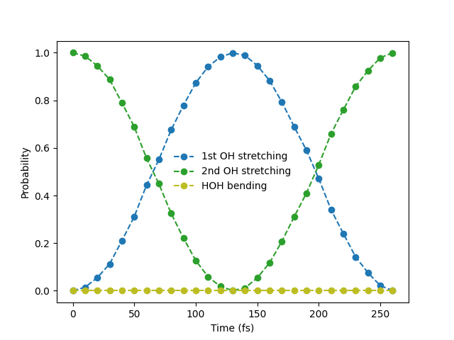
The probability of observing one vibrational quantum in the local OH modes oscillates with time. Excitations are now observed in the first local mode although this mode was not excited initially. Note that the probability of excitation in the bending mode is always zero as this mode is decoupled from the local stretching modes.

You can use the techniques outlined in this tutorial to simulate the vibrational dynamics for any input state. For instance, you can try it for a state with two vibrational quanta. The techniques can also be implemented in more sophisticated algorithms to engineer the vibrational state of a molecule.

References

1(1,2,3)

C. Sparrow, E. Martín-López, N. Maraviglia, A. Neville, C. Harrold, J. Carolan, Y. N. Joglekar, T. Hashimoto, N. Matsuda, J. L. O’Brien, D. P. Tew, and A. Laing. Simulating the Vibrational Quantum Dynamics of Molecules using Photonics. Nature, 557:660, 2018.

2(1,2)

S. Jahangiri, J. M. Arrazola, N. Quesada, and A. Delgado. Quantum Algorithm for Simulating Molecular Vibrational Excitations. arXiv, 2020.

3

C. R. Jacob and M. Reiher. Localizing Normal Modes in Large Molecules. J. Chem. Phys. 130:084106, 2009.

4

N. Killoran, J. Izaac, N. Quesada, V. Bergholm, M. Amy, and C. Weedbrook. Strawberry Fields: A Software Platform for Photonic Quantum Computing. Quantum, 3:129, 2019.

apps/run_tutorial_dynamics

 

Download Python script

 

Download Notebook