Vibrational excitations

Technical details are available in the API documentation: sf.apps.qchem.vibronic

The excitation of vibrational modes in molecules affects the outcome of chemical reactions. Vibrational excitations can provide a molecule with additional kinetic energy to overcome energy barriers of specific reaction channels and help control the stability and reactivity of the molecule [1]. However, simulating the probabilities of excitation to all vibrational levels of a molecule is challenging for processes that involve simultaneous changes in the vibrational and electronic (vibronic) states of molecules.

In this tutorial, we demonstrate how to use Gaussian Boson Sampling (GBS) to simulate molecular vibrational excitations [2]. This allows for the optimization of a vibronic process such that specific target modes of a molecule become vibrationally excited. The ability to control the final vibrational states during a vibronic process helps to engineer chemical reactions by selectively activating modes that result in preferential breaking of target chemical bonds. Let’s get started! 🧪

Vibrational excitations of pyrrole

We focus on simulating the vibrational excitations of pyrrole during a photoexcitation process. The molecule is illustrated in the figure below. Pyrrole derivatives are building blocks of important biological molecules such as chlorophyll and heme.

We first import the required modules.

import numpy as np
import strawberryfields as sf
from strawberryfields.apps import qchem
import matplotlib.pyplot as plt

We also need the molecular parameters that describe the changes in the vibrational modes and the geometry of a molecule during a vibronic transition. These are represented by the Duschinsky matrix and displacement vector [3] which are obtained from the atomic coordinates, atomic masses, vibrational frequencies, and normal modes of the molecule. These molecular parameters can be obtained from electronic structure calculations. Here, we import them as pre-computed parameters.

Li = sf.apps.data.Pyrrole(0).Li  # normal modes of the ground electronic state
Lf = sf.apps.data.Pyrrole(0).Lf  # normal modes of the excited electronic state
ri = sf.apps.data.Pyrrole(0).ri  # atomic coordinates of the ground electronic state
rf = sf.apps.data.Pyrrole(0).rf  # atomic coordinates of the excited electronic state
wi = sf.apps.data.Pyrrole(0).wi  # vibrational frequencies of the ground electronic state
wf = sf.apps.data.Pyrrole(0).wf  # vibrational frequencies of the excited electronic state
m = sf.apps.data.Pyrrole(0).m  # atomic masses

We use the duschinsky() function of the qchem module to compute the Duschinsky matrix and the displacement vector of pyrrole from the molecular data.

Ud, delta = qchem.duschinsky(Li, Lf, ri, rf, wf, m)

Let’s take a look at the Duschinsky matrix that describes the mixing of the normal modes during the vibronic transition.

plt.imshow(abs(Ud), cmap="Greens")
plt.colorbar()
plt.xlabel("Mode index")
plt.ylabel("Mode index")
plt.tight_layout()
plt.show()

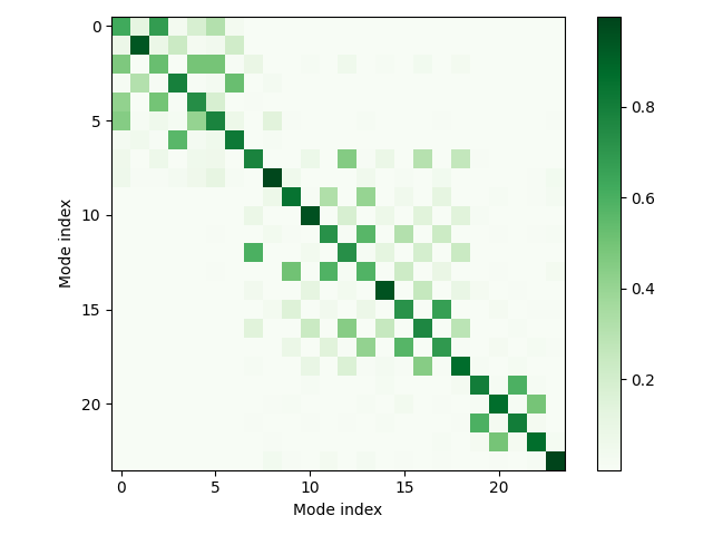
The presence of the off-diagonal entries reveals the mixing of the normal modes between different electronic states. We now compute the GBS parameters from the Duschinsky matrix and displacement vector using the gbs_params() function of the vibronic module. The first parameter generated by the gbs_params() function is needed for finite-temperature simulations which are computationally demanding. Here we restrict the simulations to zero temperature and neglect this parameter.

_, U1, r, U2, alpha = qchem.vibronic.gbs_params(wi, wf, Ud, delta)

We can now build the quantum circuit and generate five samples. The vibronic transition is simulated by applying the VibronicTransition() operation to the quantum state. This operation is equivalent to applying the Doktorov operator \(\hat{U}_{\text{Dok}} = \hat{D}({\alpha}) \hat{R}(U_2) \hat{S}({r}) \hat{R}(U_1)\) [4], which describes the transformation between the initial and the final vibronic states of a molecule when it undergoes a vibronic transition. We use the gaussian backend, which employs efficient methods for simulating GBS, and seed the random number generator to make the samples reproducible.

np.random.seed(seed=1919)
n_samples = 5
n_modes = len(alpha)
eng = sf.LocalEngine(backend="gaussian")
gbs = sf.Program(n_modes)

with gbs.context as q:
    qchem.vibronic.VibronicTransition(U1, r, U2, alpha) | q
    sf.ops.MeasureFock() | q
samples = eng.run(gbs, shots=n_samples).samples.tolist()

Out:

/opt/hostedtoolcache/Python/3.7.17/x64/lib/python3.7/site-packages/strawberryfields/backends/gaussianbackend/backend.py:216: UserWarning:

Cannot simulate non-Gaussian states. Conditional state after Fock measurement has not been updated.

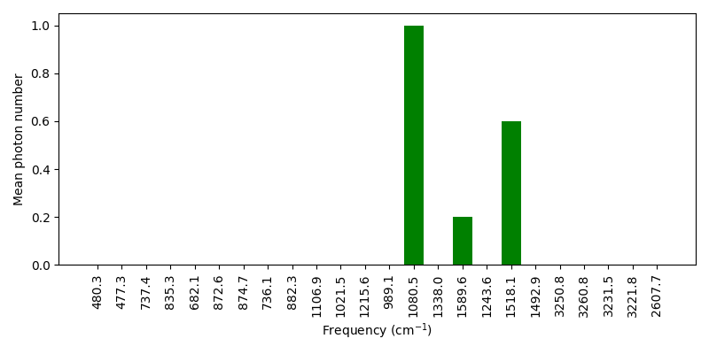
We can now compute the average number of vibrational quanta in each vibrational mode and plot the results.

n_mean = np.mean(samples, axis=0)

plt.figure(figsize=(8, 4))
plt.ylabel("Mean photon number")
plt.xlabel(r"Frequency (cm$^{-1}$)")
plt.xticks(range(len(wf)), np.round(wf, 1), rotation=90)
plt.bar(range(len(wf)), n_mean, color="green")
plt.tight_layout()
plt.show()

Let’s now simulate a photoexcitation process involving a vibronic transition from a pre-excited vibrational state of the electronic ground state. The pre-excitation step can be simulated by applying a displacement gate [2]. We insert an average number of one vibrational quantum to the OH-stretching mode (the 20th vibrational mode) and generate five samples.

np.random.seed(seed=1919)
n_samples = 5
n_modes = len(alpha)
eng = sf.LocalEngine(backend="gaussian")
gbs = sf.Program(n_modes)

with gbs.context as q:
    sf.ops.Dgate(1) | q[19]
    qchem.vibronic.VibronicTransition(U1, r, U2, alpha) | q
    sf.ops.MeasureFock() | q
samples = eng.run(gbs, shots=n_samples).samples.tolist()

We now plot the average photon numbers in each vibrational mode of the excited electronic state.

n_meanx = np.mean(samples, axis=0)

fig, ax = plt.subplots(figsize=(8, 4))
plt.ylabel("Mean photon number")
plt.xlabel(r"Frequency (cm$^{-1}$)")
plt.ylim(-1.1, 1.1)
ax.set_yticklabels([(abs(tick)) for tick in np.round(ax.get_yticks(), 1)])
ax.axhline(0, color="black", lw=0.5)
plt.xticks(range(len(wf)), np.round(wf, 1), rotation=90)
plt.bar(range(len(wf)), n_meanx, color="green", label=("input state is pre-excited"))
plt.xticks(range(len(wf)), np.round(wf, 1), rotation=90)
plt.bar(range(len(wf)), -n_mean, color="green", alpha=0.4, label=("no pre-excitation"))
plt.legend(frameon=False, loc=2)
plt.tight_layout()
plt.show()

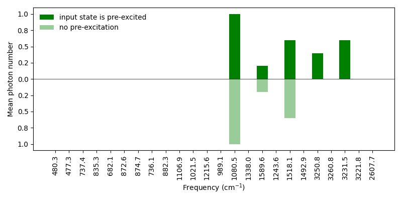
There are five excited modes now and the initial pre-excitation is transferred to two vibrational modes of the excited electronic state due to the Duschinsky mode mixing.

In this tutorial we simulated the vibrational excitations of pyrrole during vibronic transitions with GBS. This can be implemented in Strawberry Fields by writing programs that define an initial state, then apply a Doktorov transformation. Statistics of the excitations generated in each mode can be obtained by sampling repeatedly from the resulting state. This leaves significant room for exploring new configurations:

• Consider different choices of initial state. How does it affect excitations after the vibronic transition?

• How do the vibrational dynamics affect the output? Do excitations change with time?

• What other molecules can be studied?

Give it a try!

References

1

F. F. Crim. Quantum Chemical Dynamics of Vibrationally Excited Molecules: Controlling Reactions in Gases and on Surfaces. PNAS, 105:12654, 2008.

2(1,2)

S. Jahangiri, J. Miguel Arrazola, N. Quesada, and A. Delgado. Quantum Algorithm for Simulating Molecular Vibrational Excitations. arXiv, 2020.

3

F. Duschinsky. The importance of the electron spectrum in multi atomic molecules. Concerning the Franck-Condon principle. Acta Physicochim USSR, 7:551, 1937.

4

J. Huh, G. G. Guerreschi, B. Peropadre, J. R. McClean, and A. Aspuru-Guzik. Boson sampling for molecular vibronic spectra. Nature Photonics, 9:615, 2015.

apps/run_tutorial_excitations

 

Download Python script

 

Download Notebook