Minimizing the amount of correlations

Author: Nicolas Quesada

In this paper by Jiang, Lang, and Caves [1], the authors show that if one has two qumodes states \(\left|\psi \right\rangle\) and \(\left|\phi \right\rangle\) and a beamsplitter \(\text{BS}(\theta)\), then the only way no entanglement is generated when the beamsplitter acts on the product of the two states

\[\left|\Psi \right\rangle = \text{BS}(\theta) \ \left|\psi \right\rangle \otimes \left|\phi \right\rangle,\]

is if the states \(\left|\psi \right\rangle\) and \(\left|\phi \right\rangle\) are squeezed states along the same quadrature and by the same amount.

Now imagine the following task: > Given an input state \(\left|\psi \right\rangle\), which is not necessarily a squeezed state, what is the optimal state \(\left|\phi \right\rangle\) incident on a beamsplitter \(\text{BS}(\theta)\) together with \(\left|\psi \right\rangle\) such that the resulting entanglement is minimized?

In our paper we showed that if \(\theta \ll 1\) the optimal state \(\left|\phi \right\rangle\), for any input state \(\left|\psi \right\rangle\), is always a squeezed state. We furthermore conjectured that this holds for any value of \(\theta\).

Here, we numerically explore this question by performing numerical minimization over \(\left|\phi \right\rangle\) to find the state that minimizes the entanglement between the two modes.

First, we import the libraries required for this analysis; NumPy, SciPy, TensorFlow, and StrawberryFields.

import numpy as np
from scipy.linalg import expm
import tensorflow as tf

import strawberryfields as sf
from strawberryfields.ops import *
from strawberryfields.backends.tfbackend.ops import partial_trace


# set the random seed
tf.random.set_seed(137)
np.random.seed(42)

Now, we set the Fock basis truncation; in this case, we choose \(cutoff=30\):

cutoff = 30

Creating the initial states

We define our input state \(\newcommand{ket}[1]{\left|#1\right\rangle}\ket{\psi}\), an equal superposition of \(\ket{0}\) and \(\ket{1}\):

\[\ket{\psi}=\frac{1}{\sqrt{2}}\left(\ket{0}+\ket{1}\right)\]

psi = np.zeros([cutoff], dtype=np.complex128)
psi[0] = 1.0
psi[1] = 1.0
psi /= np.linalg.norm(psi)

We can now define our initial random guess for the second state \(\ket{\phi}\):

phi = np.random.random(size=[cutoff]) + 1j*np.random.random(size=[cutoff])
phi[10:] = 0.
phi /= np.linalg.norm(phi)

Next, we define the creation operator \(\hat{a}\),

a = np.diag(np.sqrt(np.arange(1, cutoff)), k=1)

the number operator \(\hat{n}=\hat{a}^\dagger \hat{a}\),

n_opt = a.T @ a

and the quadrature operators \(\hat{x}=a+a^\dagger\), \(\hat{p}=-i(a-a^\dagger)\).

# Define quadrature operators
x = a + a.T
p = -1j*(a-a.T)

We can now calculate the displacement of the states in the phase space, \(\alpha=\langle \psi \mid\hat{a}\mid\psi\rangle\). The following function calculates this displacement, and then displaces the state by \(-\alpha\) to ensure it has zero displacement.

def recenter(state):
    alpha = state.conj() @ a @ state
    disp_alpha = expm(alpha.conj()*a - alpha*a.T)
    out_state = disp_alpha @ state
    return out_state

First, let’s have a look at the displacement of state \(\ket{\psi}\) and state \(\ket{\phi}\):

print(psi.conj().T @ a @ psi)
print(phi.conj().T @ a @ phi)

Out:

(0.4999999999999999+0j)
(1.4916658938055996+0.20766920902420394j)

Now, let’s center them in the phase space:

psi = recenter(psi)
phi = recenter(phi)

Checking they now have zero displacement:

print(np.round(psi.conj().T @ a @ psi, 9))
print(np.round(phi.conj().T @ a @ phi, 9))

Out:

0j
(8e-08+1.1e-08j)

Performing the optimization

We can construct the variational quantum circuit cost function, using Strawberry Fields:

penalty_strength = 10

prog = sf.Program(2)
eng = sf.Engine("tf", backend_options={"cutoff_dim": cutoff})

psi = tf.cast(psi, tf.complex64)
phi_var_re = tf.Variable(phi.real)
phi_var_im = tf.Variable(phi.imag)


with prog.context as q:
    Ket(prog.params("input_state")) | q
    BSgate(np.pi/4, 0) | q

Here, we are initializing a TensorFlow variable phi_var representing the initial state of mode q[1], which we will optimize over. Note that we take the outer product \(\ket{in}=\ket{\psi}\otimes\ket{\phi}\), and use the Ket operator to initialise the circuit in this initial multimode pure state.

def cost(phi_var_re, phi_var_im):
    phi_var = tf.cast(phi_var_re, tf.complex64) + 1j*tf.cast(phi_var_im, tf.complex64)

    in_state = tf.einsum('i,j->ij', psi, phi_var)

    result = eng.run(prog, args={"input_state": in_state}, modes=[1])
    state = result.state

    rhoB = state.dm()
    cost = tf.cast(tf.math.real((tf.linalg.trace(rhoB @ rhoB)
                                -penalty_strength*tf.linalg.trace(rhoB @ x)**2
                                -penalty_strength*tf.linalg.trace(rhoB @ p)**2)
                           /(tf.linalg.trace(rhoB))**2), tf.float64)

    return cost

The cost function runs the engine, and we use the argument modes=[1] to return the density matrix of mode q[1].

The returned cost contains the purity of the reduced density matrix

\[\text{Tr}(\rho_B^2),\]

and an extra penalty that forces the optimized state to have zero displacement; that is, we want to minimise the value

\[\langle \hat{x}\rangle=\text{Tr}(\rho_B\hat{x}).\]

Finally, we divide by the \(\text{Tr}(\rho_B)^2\) so that the state is always normalized.

We can now set up the optimization, to minimise the cost function. Running the optimization process for 200 reps:

opt = tf.keras.optimizers.Adam(learning_rate=0.007)

reps = 200

cost_progress = []

for i in range(reps):
    # reset the engine if it has already been executed
    if eng.run_progs:
        eng.reset()

    with tf.GradientTape() as tape:
        loss = -cost(phi_var_re, phi_var_im)

    # Stores cost at each step
    cost_progress.append(loss.numpy())

    # one repetition of the optimization
    gradients = tape.gradient(loss, [phi_var_re, phi_var_im])
    opt.apply_gradients(zip(gradients, [phi_var_re, phi_var_im]))

    # Prints progress
    if i % 1 == 0:
        print("Rep: {} Cost: {}".format(i, loss))

Out:

Rep: 0 Cost: -0.4766758978366852
Rep: 1 Cost: -0.42233186960220337
Rep: 2 Cost: -0.4963145852088928
Rep: 3 Cost: -0.45958411693573
Rep: 4 Cost: -0.4818280041217804
Rep: 5 Cost: -0.5147174000740051
Rep: 6 Cost: -0.5162040591239929
Rep: 7 Cost: -0.5110472440719604
Rep: 8 Cost: -0.5209271311759949
Rep: 9 Cost: -0.5389845967292786
Rep: 10 Cost: -0.5502252578735352
Rep: 11 Cost: -0.5520217418670654
Rep: 12 Cost: -0.555342435836792
Rep: 13 Cost: -0.5651862621307373
Rep: 14 Cost: -0.5767861604690552
Rep: 15 Cost: -0.5858913660049438
Rep: 16 Cost: -0.5925743579864502
Rep: 17 Cost: -0.5986007452011108
Rep: 18 Cost: -0.6053515076637268
Rep: 19 Cost: -0.6134765148162842
Rep: 20 Cost: -0.6225422024726868
Rep: 21 Cost: -0.631293535232544
Rep: 22 Cost: -0.6387172937393188
Rep: 23 Cost: -0.6450194120407104
Rep: 24 Cost: -0.6514303684234619
Rep: 25 Cost: -0.6588231325149536
Rep: 26 Cost: -0.6668864488601685
Rep: 27 Cost: -0.6747294068336487
Rep: 28 Cost: -0.6818798780441284
Rep: 29 Cost: -0.6885322332382202
Rep: 30 Cost: -0.6950533986091614
Rep: 31 Cost: -0.7016119360923767
Rep: 32 Cost: -0.7082611918449402
Rep: 33 Cost: -0.715013861656189
Rep: 34 Cost: -0.7217400074005127
Rep: 35 Cost: -0.7281913161277771
Rep: 36 Cost: -0.7342448830604553
Rep: 37 Cost: -0.7400315999984741
Rep: 38 Cost: -0.7457356452941895
Rep: 39 Cost: -0.7513760924339294
Rep: 40 Cost: -0.7568838596343994
Rep: 41 Cost: -0.7622535824775696
Rep: 42 Cost: -0.7675090432167053
Rep: 43 Cost: -0.7726097106933594
Rep: 44 Cost: -0.7774856686592102
Rep: 45 Cost: -0.7821434140205383
Rep: 46 Cost: -0.7866564989089966
Rep: 47 Cost: -0.7910701632499695
Rep: 48 Cost: -0.7953727841377258
Rep: 49 Cost: -0.7995506525039673
Rep: 50 Cost: -0.803610622882843
Rep: 51 Cost: -0.8075515627861023
Rep: 52 Cost: -0.8113500475883484
Rep: 53 Cost: -0.8149937987327576
Rep: 54 Cost: -0.8185040950775146
Rep: 55 Cost: -0.8219097852706909
Rep: 56 Cost: -0.825222373008728
Rep: 57 Cost: -0.8284385800361633
Rep: 58 Cost: -0.8315607905387878
Rep: 59 Cost: -0.834598183631897
Rep: 60 Cost: -0.8375518918037415
Rep: 61 Cost: -0.8404152989387512
Rep: 62 Cost: -0.8431856036186218
Rep: 63 Cost: -0.8458706140518188
Rep: 64 Cost: -0.8484802842140198
Rep: 65 Cost: -0.8510206341743469
Rep: 66 Cost: -0.8534918427467346
Rep: 67 Cost: -0.8558964729309082
Rep: 68 Cost: -0.8582370281219482
Rep: 69 Cost: -0.8605165481567383
Rep: 70 Cost: -0.8627358675003052
Rep: 71 Cost: -0.8648964762687683
Rep: 72 Cost: -0.8670018315315247
Rep: 73 Cost: -0.8690568208694458
Rep: 74 Cost: -0.8710666298866272
Rep: 75 Cost: -0.8730332255363464
Rep: 76 Cost: -0.8749582767486572
Rep: 77 Cost: -0.87684166431427
Rep: 78 Cost: -0.8786839842796326
Rep: 79 Cost: -0.8804851174354553
Rep: 80 Cost: -0.8822448253631592
Rep: 81 Cost: -0.883963942527771
Rep: 82 Cost: -0.8856426477432251
Rep: 83 Cost: -0.8872805237770081
Rep: 84 Cost: -0.888877809047699
Rep: 85 Cost: -0.8904345035552979
Rep: 86 Cost: -0.8919485807418823
Rep: 87 Cost: -0.8934181928634644
Rep: 88 Cost: -0.8948407769203186
Rep: 89 Cost: -0.8962131142616272
Rep: 90 Cost: -0.8975301384925842
Rep: 91 Cost: -0.8987881541252136
Rep: 92 Cost: -0.8999797701835632
Rep: 93 Cost: -0.9011000990867615
Rep: 94 Cost: -0.9021427631378174
Rep: 95 Cost: -0.9031028151512146
Rep: 96 Cost: -0.9039767980575562
Rep: 97 Cost: -0.9047643542289734
Rep: 98 Cost: -0.9054700136184692
Rep: 99 Cost: -0.9061008095741272
Rep: 100 Cost: -0.9066663384437561
Rep: 101 Cost: -0.9071784019470215
Rep: 102 Cost: -0.9076470136642456
Rep: 103 Cost: -0.9080800414085388
Rep: 104 Cost: -0.908480703830719
Rep: 105 Cost: -0.9088495373725891
Rep: 106 Cost: -0.9091846346855164
Rep: 107 Cost: -0.9094841480255127
Rep: 108 Cost: -0.9097475409507751
Rep: 109 Cost: -0.9099751710891724
Rep: 110 Cost: -0.9101700186729431
Rep: 111 Cost: -0.910335898399353
Rep: 112 Cost: -0.9104783535003662
Rep: 113 Cost: -0.9106017351150513
Rep: 114 Cost: -0.9107117056846619
Rep: 115 Cost: -0.9108109474182129
Rep: 116 Cost: -0.9109016060829163
Rep: 117 Cost: -0.9109863638877869
Rep: 118 Cost: -0.9110652804374695
Rep: 119 Cost: -0.9111390709877014
Rep: 120 Cost: -0.9112085700035095
Rep: 121 Cost: -0.9112733006477356
Rep: 122 Cost: -0.9113340377807617
Rep: 123 Cost: -0.9113907814025879
Rep: 124 Cost: -0.9114443063735962
Rep: 125 Cost: -0.9114949107170105
Rep: 126 Cost: -0.9115434288978577
Rep: 127 Cost: -0.9115898013114929
Rep: 128 Cost: -0.9116342067718506
Rep: 129 Cost: -0.911677360534668
Rep: 130 Cost: -0.9117187857627869
Rep: 131 Cost: -0.9117587804794312
Rep: 132 Cost: -0.9117969274520874
Rep: 133 Cost: -0.9118332862854004
Rep: 134 Cost: -0.9118677377700806
Rep: 135 Cost: -0.9118999242782593
Rep: 136 Cost: -0.91193026304245
Rep: 137 Cost: -0.9119580388069153
Rep: 138 Cost: -0.9119839072227478
Rep: 139 Cost: -0.9120075106620789
Rep: 140 Cost: -0.9120290279388428
Rep: 141 Cost: -0.91204833984375
Rep: 142 Cost: -0.9120662808418274
Rep: 143 Cost: -0.9120829701423645
Rep: 144 Cost: -0.9120978713035583
Rep: 145 Cost: -0.9121111631393433
Rep: 146 Cost: -0.9121232628822327
Rep: 147 Cost: -0.9121341705322266
Rep: 148 Cost: -0.9121443033218384
Rep: 149 Cost: -0.9121530055999756
Rep: 150 Cost: -0.9121609926223755
Rep: 151 Cost: -0.9121681451797485
Rep: 152 Cost: -0.9121743440628052
Rep: 153 Cost: -0.9121801853179932
Rep: 154 Cost: -0.9121854305267334
Rep: 155 Cost: -0.9121900796890259
Rep: 156 Cost: -0.912194550037384
Rep: 157 Cost: -0.9121983051300049
Rep: 158 Cost: -0.9122019410133362
Rep: 159 Cost: -0.9122051000595093
Rep: 160 Cost: -0.9122082591056824
Rep: 161 Cost: -0.9122109413146973
Rep: 162 Cost: -0.9122136235237122
Rep: 163 Cost: -0.9122157692909241
Rep: 164 Cost: -0.9122180342674255
Rep: 165 Cost: -0.912219762802124
Rep: 166 Cost: -0.912221372127533
Rep: 167 Cost: -0.9122230410575867
Rep: 168 Cost: -0.912224292755127
Rep: 169 Cost: -0.9122257828712463
Rep: 170 Cost: -0.9122268557548523
Rep: 171 Cost: -0.9122277498245239
Rep: 172 Cost: -0.9122288227081299
Rep: 173 Cost: -0.9122294187545776
Rep: 174 Cost: -0.9122301340103149
Rep: 175 Cost: -0.9122310280799866
Rep: 176 Cost: -0.9122319221496582
Rep: 177 Cost: -0.9122321009635925
Rep: 178 Cost: -0.9122328758239746
Rep: 179 Cost: -0.912233293056488
Rep: 180 Cost: -0.9122336506843567
Rep: 181 Cost: -0.9122341275215149
Rep: 182 Cost: -0.9122345447540283
Rep: 183 Cost: -0.9122346043586731
Rep: 184 Cost: -0.9122349619865417
Rep: 185 Cost: -0.9122350215911865
Rep: 186 Cost: -0.9122353792190552
Rep: 187 Cost: -0.9122354388237
Rep: 188 Cost: -0.9122354984283447
Rep: 189 Cost: -0.9122358560562134
Rep: 190 Cost: -0.9122357964515686
Rep: 191 Cost: -0.9122359156608582
Rep: 192 Cost: -0.9122359156608582
Rep: 193 Cost: -0.9122361540794373
Rep: 194 Cost: -0.912236213684082
Rep: 195 Cost: -0.912236213684082
Rep: 196 Cost: -0.9122361540794373
Rep: 197 Cost: -0.9122360944747925
Rep: 198 Cost: -0.912236213684082
Rep: 199 Cost: -0.9122360944747925

We can see that the optimization converges to the optimum purity value of 0.9122365.

Visualising the optimum state

We can now calculate the density matrix of the input state \(\ket{\phi}\) which minimises entanglement:

\[\rho_{\phi} = \ket{\phi}\left\langle \phi\right|\]

ket_val = phi_var_re.numpy() + phi_var_im.numpy()*1j
out_rhoB = np.outer(ket_val, ket_val.conj())
out_rhoB /= np.trace(out_rhoB)

Note that the optimization is not guaranteed to keep the state normalized, so we renormalize the minimized state.

Next, we can use the following function to plot the Wigner function of this density matrix:

import copy
def wigner(rho, xvec, pvec):
    # Modified from qutip.org
    Q, P = np.meshgrid(xvec, pvec)
    A = (Q + P * 1.0j) / (2 * np.sqrt(2 / 2))

    Wlist = np.array([np.zeros(np.shape(A), dtype=complex) for k in range(cutoff)])

    # Wigner function for |0><0|
    Wlist[0] = np.exp(-2.0 * np.abs(A) ** 2) / np.pi

    # W = rho(0,0)W(|0><0|)
    W = np.real(rho[0, 0]) * np.real(Wlist[0])

    for n in range(1, cutoff):
        Wlist[n] = (2.0 * A * Wlist[n - 1]) / np.sqrt(n)
        W += 2 * np.real(rho[0, n] * Wlist[n])

    for m in range(1, cutoff):
        temp = copy.copy(Wlist[m])
        # Wlist[m] = Wigner function for |m><m|
        Wlist[m] = (2 * np.conj(A) * temp - np.sqrt(m)
                    * Wlist[m - 1]) / np.sqrt(m)

        # W += rho(m,m)W(|m><m|)
        W += np.real(rho[m, m] * Wlist[m])

        for n in range(m + 1, cutoff):
            temp2 = (2 * A * Wlist[n - 1] - np.sqrt(m) * temp) / np.sqrt(n)
            temp = copy.copy(Wlist[n])
            # Wlist[n] = Wigner function for |m><n|
            Wlist[n] = temp2

            # W += rho(m,n)W(|m><n|) + rho(n,m)W(|n><m|)
            W += 2 * np.real(rho[m, n] * Wlist[n])

    return Q, P, W / 2

# Import plotting
from matplotlib import pyplot as plt
# %matplotlib inline

x = np.arange(-5, 5, 0.1)
p = np.arange(-5, 5, 0.1)
X, P, W = wigner(out_rhoB, x, p)
plt.contourf(X, P, np.round(W,3), cmap="PiYG")
plt.show()

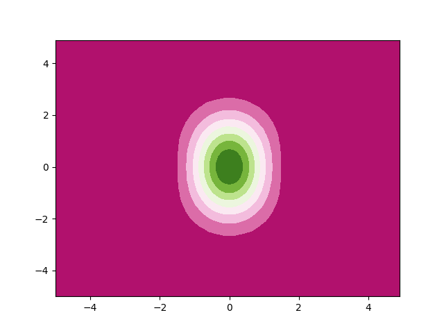
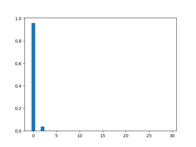
We see that the optimal state is indeed a (mildly) squeezed state. This can be confirmed by visuallising the Fock state probabilities of state \(\ket{\phi}\):

plt.bar(np.arange(cutoff), height=np.diag(out_rhoB).real)
plt.show()

Finally, printing out the mean number of photons \(\bar{n} = \left\langle \phi \mid \hat{n} \mid \phi\right\rangle = \text{Tr}(\hat{n}\rho)\), as well as the squeezing magnitude \(r=\sinh^{-1}\left(\sqrt{\bar{n}}\right)\) of this state:

nbar = np.trace(n_opt @ out_rhoB).real
print("mean number of photons =", nbar)
print("squeezing parameter =", np.arcsinh(np.sqrt(nbar)))

Out:

mean number of photons = 0.08352928524073516
squeezing parameter = 0.2851349275051653

References

[1] Jiang, Z., Lang, M. D., & Caves, C. M. (2013). Mixing nonclassical pure states in a linear-optical network almost always generates modal entanglement. Physical Review A, 88(4), 044301.

[2] Quesada, N., & Brańczyk, A. M. (2018). Gaussian functions are optimal for waveguided nonlinear-quantum-optical processes. Physical Review A, 98, 043813.

demos/run_minimizing_correlations

 

Download Python script

 

Download Notebook