Note
Click here to download the full example code
Scattershot Boson Sampling
Author: Arthur Pesah
Implementation of Scattershot Boson Sampling (see references (1) and (2)) in Strawberry Fields.
As we have seen in the Boson Sampling (BS) tutorial, a boson sampler is a quantum machine that takes a deterministic input made of \(m\) modes, \(n\) of them sending photons simultaneously through an interferometer modeled by a unitary matrix \(U\). The output of the interferometer is a random distribution of photons that can be computed classically with the permanent of \(U\).
Scattershot Boson Sampling (SBS) was motivated by the fact that emitting \(n\) photons simultaneously in the input is experimentally very hard to realize for large \(n\). What is simpler to build is a random input using Spontaneous Parametric Down-Conversion (SPDC), whose distribution is given by \(P(k_i = k)=(1-\chi^2) \chi^{2 k}\) where \(k_i\) is the number of photon in mode i and \(\chi \in (-1,1)\) is a given parameter (equation (7) of the original paper (1)). The advantage of SPDC is not only that it’s a coherent source of photons but also that it always emits an even number of photons: one that can be used in a boson sampling circuit and one to measure the input.
In quantum optics, we model SPDC by 2-mode squeezing gates \(\hat{S}_2\) such that \(\hat{S}_2 |0 \rangle |0 \rangle = \sqrt{(1-\chi^2)} \sum_{k=0}^{\infty} \chi^k |k \rangle |k \rangle\) (equation (3) of the paper). The first qumode will be used to measure the input while the second will be sent to the circuit.
In SF, this 2-mode squeezing gate is called the S2gate and takes as
input a squeezing parameter \(r\) related to \(\chi\) by the
formula \(r=\tanh(\chi)\).
import numpy as np
import scipy as sp
from math import factorial, tanh
import itertools

import matplotlib.pyplot as plt
# %matplotlib inline
import matplotlib.path as mpath
import matplotlib.lines as mlines
import matplotlib.patches as mpatches
from matplotlib.collections import PatchCollection

import strawberryfields as sf
from strawberryfields.ops import *

colormap = np.array(plt.rcParams['axes.prop_cycle'].by_key()['color'])
Constructing the circuit
Constants
Our circuit will depend on a few parameters. The first constants are the squeezing parameter \(r \in [-1,1]\) (already described in introduction) and the cutoff number, which corresponds to the maximum number of photons per mode considered in the computation (used to make the simulation tractable).
r_squeezing = 0.5 # squeezing parameter for the S2gate (here taken randomly between -1 and 1)
cutoff = 7 # max number of photons computed per mode
Then comes the unitary matrix, representing the interferometer. We have decided to implement a 4-modes boson sampler, and we therefore need a \(4 \times 4\)-unitary matrix. Any kind of such unitary matrix could do well, but for simplicity, we choose to implement it using two rotations: one with angle \(\theta_1\) for the qumodes 1 and 2, and another with angle \(\theta_2\) for the qubits 3 and 4. The final matrix has the form:
theta1 = 0.5
theta2 = 1

U = np.array([[np.cos(theta1), -np.sin(theta1), 0,               0             ],
              [np.sin(theta1),  np.cos(theta1), 0,               0             ],
              [0,               0,              np.cos(theta2), -np.sin(theta2)],
              [0,               0,              np.sin(theta2),  np.cos(theta2)]])
Circuit
We instantiate our circuit with 8 qubits, 4 for the input, 4 for the output.
prog = sf.Program(8)
We can then declare our circuit. The first four lines are 2-modes squeezing gates, which generate a random number of photons
with prog.context as q:
    S2gate(r_squeezing) | (q[0], q[4])
    S2gate(r_squeezing) | (q[1], q[5])
    S2gate(r_squeezing) | (q[2], q[6])
    S2gate(r_squeezing) | (q[3], q[7])

    Interferometer(U) | (q[4], q[5], q[6], q[7])
Running
Run the simulation up to ‘cutoff’ photons per mode
Out:
/opt/hostedtoolcache/Python/3.7.17/x64/lib/python3.7/site-packages/strawberryfields/program.py:661: UserWarning: The circuit consists of 2 disconnected components.
Get the probability associated to each state
probs = state.all_fock_probs()
Reshape ‘probs’ such that probs \([m_1, \dots, m_4,n_1, \dots, n_4]\) gives the probability of the having jointly the input state \((m_1, \dots, m_4)\) (with \(m_i\) the number of photons in input mode \(i\)) and the output state \((n_1, \dots, n_4)\) (with \(n_i\) the number of photons in output mode \(i\))
probs = probs.reshape(*[cutoff]*8)
The sum is not 1 because of the finite cutoff:
np.sum(probs)
Out:
0.9998583445961168
Analysis
The goal of this section is to compare the simulated probability with the theoretical one.
Computation of the theoretical probability
To do so, the first step is to compute the theoretical probability \(P(\mathrm{input}=(m_1, m_2, m_3, m_4), \mathrm{output}=(n_1, n_2, n_3, n_4))\), where \(m_i,n_i \in \mathbb{N}\) represent the number of photons respectively in input and output modes \(i\). Using the definition of conditional probability, we can decompose it as:
The value of \(P(\mathrm{output} \mid \mathrm{input})\) is given in the Boson Sampling tutorial:
while \(P(\mathrm{input})\) depends on the SPDC properties (see introduction) and can be computed in the following way:
with \(m\) the number of modes (here 4) and \(n=\sum m_i\) the total number of photons. The value of \(P(m_i)\) is directly taken from the original paper (equation (7)).
Using that, we can now perform the computation.
First, the permanent of the matrix can be calculated via The Walrus library:
from thewalrus import perm
Then the probability of the output given an input. For that, we use the algorithm given in section V of reference (3) to compute the matrix \(U_{st}\) (called \(U_{I,O}\) in the cited paper). To sum it up, it consists in extracting \(m_j\) times the column \(j\) of \(U\) for every \(j\), and \(n_i\) times the row \(i\) of \(U\) for every \(i\) (with \(m_j\) and \(n_i\) still representing the number of photons respectively in input \(j\) and output \(i\)).
def get_proba_output(U, input, output):
    # The two lines below are the extracted row and column indices.
    # For instance, for output=[3,2,1,0], we want list_rows=[0,0,0,1,1,2].
    # sum(.,[]) is a Python trick to flatten the list
    list_rows = sum([[i] * output[i] for i in range(len(output))],[])
    list_columns = sum([[i] * input[i] for i in range(len(input))],[])

    U_st = U[:,list_columns][list_rows,:]
    perm_squared = np.abs(perm(U_st, method="ryser"))**2
    denominator = np.prod([factorial(inp) for inp in input]) * np.prod([factorial(out) for out in output])
    return perm_squared / denominator

def get_proba_input(input):
    chi = np.tanh(r_squeezing)
    n = np.sum(input)
    m = len(input)
    return (1 - chi**2)**m * chi**(2*n)

def get_proba(U, result):
    input, output = result[0:4], result[4:8]
    return get_proba_output(U, input, output) * get_proba_input(input) # P(O,I) = P(O|I) P(I)
Comparison between theory and simulation
print("Theory: \t", get_proba(U, [0,0,0,0,0,0,0,0]))
print("Simulation: \t", probs[0,0,0,0,0,0,0,0])

print("Theory: \t", get_proba(U, [1,0,0,0,1,0,0,0]))
print("Simulation: \t", probs[1,0,0,0,1,0,0,0])

print("Theory: \t", get_proba(U, [1,0,0,0,0,1,0,0]))
print("Simulation: \t", probs[1,0,0,0,0,1,0,0])
Out:
Theory:          0.3825422953821255
Simulation:      0.3825422953821258
Theory:          0.06291578440230364
Simulation:      0.06291578440230369
Theory:          0.018776990012967093
Simulation:      0.018776990012967107
We see that the results are very similar.
Visualization
To visualize the results and the effect of a scattershot boson sampler, we will draw some examples of sampling.
Make the probabilities sum to 1
Due to computational issues, the sum of the probability does not equal 1. Since it prevents us from sampling correctly, we choose to add the missing weight to the outcome [0,0,0,0, 0,0,0,0]
probs[0,0,0,0, 0,0,0,0] += 1 - np.sum(probs)

np.sum(probs)
Out:
1.0
Sample
Get all possible choices as a list of outcomes \([m_1, m_2, m_3, m_4, n_1, n_2, n_3, n_4 ]\)
list_choices = list(itertools.product(*[range(cutoff)]*8))
list_choices[0]
Out:
(0, 0, 0, 0, 0, 0, 0, 0)
Get the probability of each choice index
list_probs = [probs[list_choices[i]] for i in range(len(list_choices))]
list_probs[0]
Out:
0.38268395078600903
Sample a choice using this probability distribution
choice = list_choices[np.random.choice(range(len(list_choices)), p=list_probs)]
choice
Out:
(1, 1, 1, 0, 2, 0, 0, 1)
Visualize
Constants
## Colors
color_interf = colormap[0]
color_lines = "black"
color_laser = colormap[3]
color_photons = "#F5D76E"
color_spdc = colormap[4]
color_meas = colormap[1]

color_text_interf = "white"
color_text_spdc = "white"
color_text_measure = "white"

## Sizes
unit = 0.05
radius_photons = 0.015
margin_photons = 0.01
margin_input_meas = 1*unit # space between the end of the input measure and the interferometer

width_laser = 8*unit
width_spdc = 2*unit
width_lines_spdc = 1*unit
width_line_interf = 8*unit
width_measure = 2*unit
width_line_input = width_line_interf - margin_input_meas - width_measure
width_interf = 8*unit
width_line_output = 6*unit

height_interf = 20*unit
height_spdc = 2*unit

## Positions
x_begin_laser = -0.5
x_begin_spdc = x_begin_laser + width_laser
x_end_spdc = x_begin_spdc + width_spdc
x_begin_lines_spdc = x_end_spdc
x_end_lines_spdc = x_end_spdc + width_lines_spdc
x_end_line_input = x_end_lines_spdc + width_line_input
x_begin_input_meas = x_end_line_input
x_end_input_meas = x_begin_input_meas + width_measure
x_begin_interf = x_end_lines_spdc + width_line_interf
x_end_interf = x_begin_interf + width_interf
x_end_line_output = x_end_interf + width_line_output
x_end_output_meas = x_end_line_output + width_measure

y_begin_interf = 0
sep_lines_interf = height_interf / 5
sep_lines_spdc = 2*unit
Plot
# Sampling

choice = list_choices[np.random.choice(range(len(list_choices)), p=list_probs)]

# Plot

fig, ax = plt.subplots()
fig.set_size_inches(12, 9)
fig.axis = "equal"

interf = mpatches.Rectangle((x_begin_interf,0),width_interf, height_interf,
                            edgecolor=color_interf,facecolor=color_interf)
ax.add_patch(interf)

plt.text(x_begin_interf+width_interf/2, y_begin_interf+height_interf/2, 'U',
         {'ha': 'center', 'va': 'center'}, size=40, color=color_text_interf)

for i_line in range(4):
    y_line_interf = y_begin_interf + (i_line+1) * sep_lines_interf
    y_line_input = y_line_interf + sep_lines_spdc
    y_line_laser = y_line_interf + (y_line_input - y_line_interf) / 2

    # draw laser lines
    plt.plot([x_begin_laser,x_begin_spdc], [y_line_laser,y_line_laser], color=color_laser)

    # draw lines for the output of the SPDC
    plt.plot([x_begin_lines_spdc,x_end_lines_spdc], [y_line_laser,y_line_interf], color=color_lines)
    plt.plot([x_begin_lines_spdc,x_end_lines_spdc], [y_line_laser,y_line_input], color=color_lines)

    # draw lines interferometer lines
    plt.plot([x_end_lines_spdc,x_begin_interf], [y_line_interf,y_line_interf], color=color_lines)
    plt.plot([x_end_interf, x_end_line_output], [y_line_interf,y_line_interf], color=color_lines)

    # draw lines for the input photons (before measure)
    plt.plot([x_end_lines_spdc,x_end_line_input], [y_line_input,y_line_input], color=color_lines)

    # draw the input measures
    input_meas = mpatches.Rectangle((x_begin_input_meas, y_line_input-width_measure/2),width_measure,width_measure,
                                    edgecolor=color_meas,facecolor=color_meas)
    plt.text(x_begin_input_meas+width_measure/2, y_line_input, str(choice[i_line]),
             {'ha': 'center', 'va': 'center'}, size=12, color=color_text_measure)
    ax.add_patch(input_meas)

    # draw the output measures
    input_meas = mpatches.Rectangle((x_end_line_output, y_line_interf-width_measure/2),width_measure,width_measure,
                                    edgecolor=color_meas,facecolor=color_meas)
    plt.text(x_end_line_output+width_measure/2, y_line_interf, str(choice[4+i_line]),
             {'ha': 'center', 'va': 'center'}, size=12, color=color_text_measure)
    ax.add_patch(input_meas)

    # draw the SPDC
    spdc = mpatches.Rectangle((x_begin_spdc,y_line_interf),width_spdc,height_spdc,
                              edgecolor=color_spdc,facecolor=color_spdc, zorder=3)
    plt.text(x_begin_spdc+width_spdc/2, y_line_interf+height_spdc/2, 'SPDC',
             {'ha': 'center', 'va': 'center'}, size=12, color=color_text_spdc)
    ax.add_patch(spdc)

    # draw the input photons
    for i_photon in range(choice[i_line]):
        x_photon = x_end_line_input - margin_photons - radius_photons - i_photon*(radius_photons*2 + margin_photons)
        circle = mpatches.Circle([x_photon,y_line_input], radius_photons, color=color_photons, zorder=3)
        ax.add_patch(circle)

    # draw the output photons
    for i_photon in range(choice[4 + i_line]):
        x_photon = x_end_line_output - margin_photons - radius_photons - i_photon*(radius_photons*2 + margin_photons)
        circle = mpatches.Circle([x_photon,y_line_interf], radius_photons, color=color_photons, zorder=3)
        ax.add_patch(circle)

plt.title("Choice: {}".format(choice))
plt.axis('equal')
plt.axis('off')
Out:
(-0.5875, 1.3375000000000004, -0.05, 1.05)
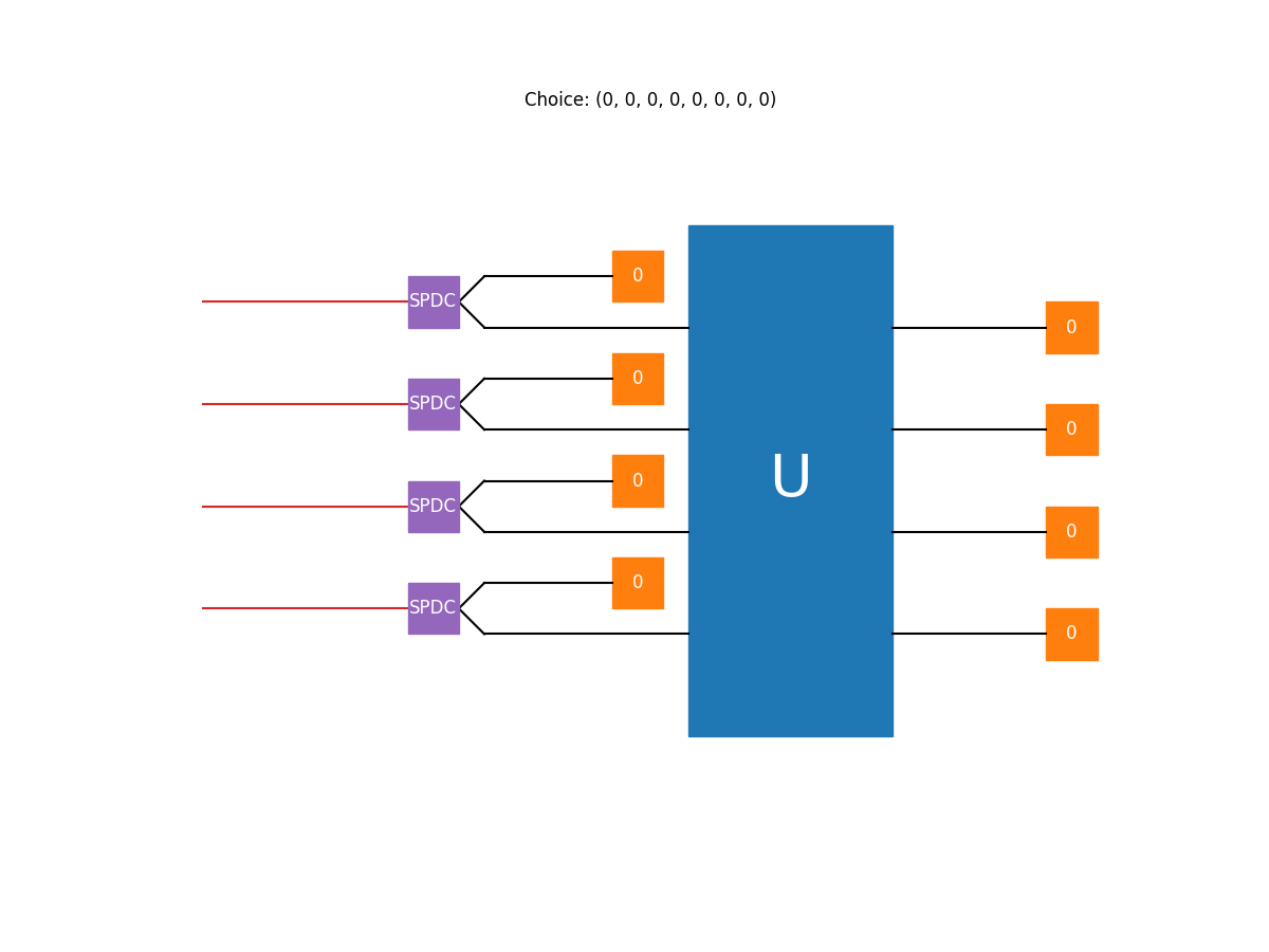
This figure represents an example of sampling (each time you execute the cell, it samples a new state).
At time 0, a laser hits the 4 SPDC, which produce in consequence \(n\) pairs of photons. For each pair, one photon is sent to a measuring device (for the input) and the other to the interferometer. This interferometer then outputs those \(n\) photons, but in different modes (different lines in the figure), following the probability distribution described above. A measuring device finally captures those output photons.
A state consists of both the input photons (produced by the SPDC) and the output ones.
References
A. P. Lund, A. Laing, S. Rahimi-Keshari, T. Rudolph, J. L O’Brien and T. C. Ralph. Boson Sampling from Gaussian States. Physical Review Letters, doi:10.1103/PhysRevLett.113.100502.
Scott Aaronson. Scattershot Boson Sampling: A new approach to scalable Boson Sampling experiments. Blog article.
Max Tillmann, Borivoje Dakić, René Heilmann, Stefan Nolte, Alexander Szameit, Philip Walther. Experimental Boson Sampling. Nature Photonics doi:10.1038/nphoton.2013.102.
Total running time of the script: ( 0 minutes 8.415 seconds)
Contents
Downloads
Related tutorials