Sampling quadratures of non-Gaussian states using the bosonic backend

Note

This tutorial is second in a series on the bosonic backend. For an introduction to the backend, see part 1. Once finished this tutorial, check out part 3 for a deep dive into using the bosonic backend to simulate qubits encoded in photonic modes. These tutorials accompany our research paper [1].

In a previous tutorial we introduced the bosonic backend, the fourth and latest software backend of Strawberry Fields. In this tutorial we continue investigating some of its functionality by exploring how to sample quadrature (homodyne) measurements in non-Gaussian states. While these simulations could be done in the fock backend, it is a lot more convenient to use the new backend, since simulations in the fock backend need to remain under an energy cutoff.

We first return to our old friend, the cat state, and see how it looks when projected (measured) along different quadratures of phase space. Then we investigate a useful class of non-Gaussian states known as grid or GKP states. These states are named after Daniel Gottesman , Alexei Kitaev and John Preskill who introduced them in a seminal paper in 2001 [2].

Cat quadratures

In a previous tutorial we investigated the Wigner function of the cat state. Now, we will explore the distributions of its quadratures. The distributions of the position \(q\) and momentum \(p\) quadratures can be obtained by integrating the Wigner function:

\[\begin{split}\text{Pr}(q=x) = \int_{-\infty}^\infty dp~ W(x,p), \\ \text{Pr}(p=y) = \int_{-\infty}^\infty dq~ W(q,y).\end{split}\]

Note that even though the Wigner function can be negative (as it is a quasiprobability distribution), the quadrature distributions \(\text{Pr}(q=x)\) and \(\text{Pr}(p=y)\) are proper probability distributions, i.e., they are non-negative and their integrals equal unity.

We will use Strawberry Fields to investigate how these distributions look for a cat state.

# We do the usual imports
import strawberryfields as sf
import numpy as np
import matplotlib.pyplot as plt
import matplotlib as mpl
from matplotlib import cm

# Create cat state
prog_cat = sf.Program(1)

with prog_cat.context as q:
    sf.ops.Catstate(a=2) | q

eng = sf.Engine("bosonic")
cat = eng.run(prog_cat).state

Strawberry Fields provides handy functions for accessing the quadrature distributions. These can retrieved using the marginal method of the state object:

# Calculate the quadrature distributions
scale = np.sqrt(sf.hbar)
quad_axis= np.linspace(-6, 6, 1000) * scale
cat_prob_x = cat.marginal(0, quad_axis)  # This is the q quadrature
cat_prob_p = cat.marginal(0, quad_axis, phi=np.pi / 2)  # This is the p quadrature

We can also use Strawberry Fields to generate samples of a given quadrature. In this case, we do it for the \(q\) quadrature:

# Run the program again, collecting q samples this time
shots = 2000  # Number of samples
prog_cat_x = sf.Program(1)

with prog_cat_x.context as q:
    sf.ops.Catstate(a=2) | q
    sf.ops.MeasureX | q

eng = sf.Engine("bosonic")
cat_samples_x = eng.run(prog_cat_x, shots=shots).samples[:, 0]

We can also sample the \(p\) quadrature:

# Run the program again, collecting p samples this time
prog_cat_p = sf.Program(1)

with prog_cat_p.context as q:
    sf.ops.Catstate(a=2) | q
    sf.ops.MeasureP | q

eng = sf.Engine("bosonic")
cat_samples_p = eng.run(prog_cat_p, shots=shots).samples[:, 0]

We can verify that the samples distribute according to the expected distribution:

# Plot the results
fig, axs = plt.subplots(1, 2, figsize=(10, 4))
fig.suptitle(r"$|0^{\alpha}\rangle_{cat}$, $\alpha=2$", fontsize=18)

axs[0].hist(cat_samples_x / scale, bins=100, density=True, label="Samples", color="cornflowerblue")
axs[0].plot(quad_axis/ scale, cat_prob_x * scale, "--", label="Ideal", color="tab:red")
axs[0].set_xlabel(r"q (units of $\sqrt{\hbar}$)", fontsize=15)
axs[0].set_ylabel("Pr(q)", fontsize=15)

axs[1].hist(cat_samples_p / scale, bins=100, density=True, label="Samples", color="cornflowerblue")
axs[1].plot(quad_axis/ scale, cat_prob_p * scale, "--", label="Ideal", color="tab:red")
axs[1].set_xlabel(r"p (units of $\sqrt{\hbar}$)", fontsize=15)
axs[1].set_ylabel("Pr(p)", fontsize=15)

axs[1].legend()
axs[0].tick_params(labelsize=13)
axs[1].tick_params(labelsize=13)
fig.tight_layout(rect=[0, 0.03, 1, 0.95])
plt.show()

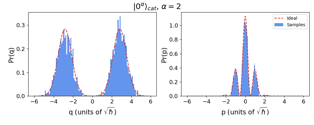
As we can see, we obtain a positive-valued probability distribution. The two lobes arising from the coherent states superposed in the cat state are clearly visible in \(q\) distribution.

GKP quadratures

As mentioned before, the bosonic backend can easily handle a number of nonclassical states of light. A particularly useful family of states are the so-called GKP or grid states. In the same way that cat states are linear superpositions of two coherent states, GKP states can be understood as superpositions of multiple squeezed states. We can generate a GKP state and plot its Wigner function using Strawberry Fields in the same way we did for cat states.

# Create GKP state
epsilon = 0.1
prog_gkp = sf.Program(1)
with prog_gkp.context as q:
    sf.ops.GKP(epsilon=epsilon) | q
eng = sf.Engine("bosonic")
gkp = eng.run(prog_gkp).state

Wgkp = gkp.wigner(mode=0, xvec=quad_axis, pvec=quad_axis)
scale = np.max(Wgkp.real)
nrm = mpl.colors.Normalize(-scale, scale)
plt.axes().set_aspect("equal")
plt.contourf(quad_axis, quad_axis, Wgkp, 60, cmap=cm.RdBu, norm=nrm)
plt.xlabel(r"q (units of $\sqrt{\hbar}$)", fontsize=15)
plt.ylabel(r"p (units of $\sqrt{\hbar}$)", fontsize=15)
plt.tight_layout()
plt.show()

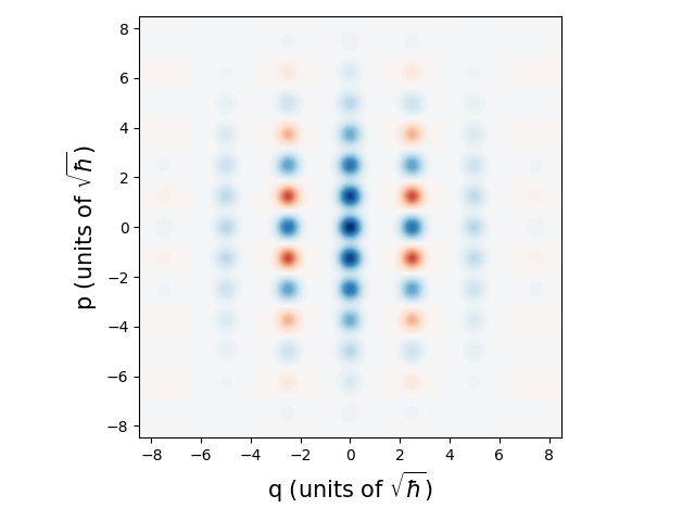
We see that GKP states in phase space are made of multiple narrow peaks of alternating signs. After getting an idea of how a GKP state looks in phase-space we can now turn our attention to understanding its quadrature distribution.

# As before, we can directly calculate the expected quadrature distributions
scale = np.sqrt(sf.hbar * np.pi)
quad_axis= np.linspace(-6, 6, 1000) * scale
gkp_prob_x = gkp.marginal(0, quad_axis)
gkp_prob_p = gkp.marginal(0, quad_axis, phi=np.pi / 2)

Like before, we can collect samples of the quadratures to simulate the state being probed with homodyne measurements:

# Run the program again, collecting q samples this time
prog_gkp_x = sf.Program(1)
with prog_gkp_x.context as q:
    sf.ops.GKP(epsilon=0.1) | q
    sf.ops.MeasureX | q
eng = sf.Engine("bosonic")
gkp_samples_x = eng.run(prog_gkp_x, shots=shots).samples[:, 0]

# Run the program again, collecting p samples this time
prog_gkp_p = sf.Program(1)
with prog_gkp_p.context as q:
    sf.ops.GKP(epsilon=0.1) | q
    sf.ops.MeasureP | q
eng = sf.Engine("bosonic")
gkp_samples_p = eng.run(prog_gkp_p, shots=shots).samples[:, 0]

and can compare the results:

# Plot the results
fig, axs = plt.subplots(1, 2, figsize=(10, 4))
fig.suptitle(r"$|0^\epsilon\rangle_{GKP}$, $\epsilon=0.1$ (10 dB)", fontsize=18)

axs[0].hist(gkp_samples_x / scale, bins=100, density=True, label="Samples", color="cornflowerblue")
axs[0].plot(quad_axis/ scale, gkp_prob_x * scale, "--", label="Ideal", color="tab:red")
axs[0].set_xlabel(r"q (units of $\sqrt{\pi\hbar}$)", fontsize=15)
axs[0].set_ylabel("Pr(q)", fontsize=15)

axs[1].hist(gkp_samples_p / scale, bins=100, density=True, label="Samples", color="cornflowerblue")
axs[1].plot(quad_axis/ scale, gkp_prob_p * scale, "--", label="Ideal", color="tab:red")
axs[1].set_xlabel(r"p (units of $\sqrt{\pi\hbar}$)", fontsize=15)
axs[1].set_ylabel("Pr(p)", fontsize=15)

axs[1].legend()
axs[0].tick_params(labelsize=13)
axs[1].tick_params(labelsize=13)
fig.tight_layout(rect=[0, 0.03, 1, 0.95])
plt.show()

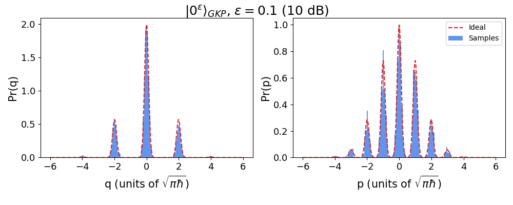
The comb of peaks are clearly visible in both the quadratures, as are visible the Gaussian spread of the individual peaks and the Gaussian envelope on the height of all the peaks.

Conclusion and Outlook

In this tutorial we have explored the sampling functionality of the bosonic backend by investigating the quadrature distributions of both cat and GKP states. For advanced readers, we encourage you to read part 3 to take a dive into how GKP states can be used to encode a qubit in a photonic mode.

References

1

J. Eli Bourassa, Nicolás Quesada, Ilan Tzitrin, Antal Száva, Theodor Isacsson, Josh Izaac, Krishna Kumar Sabapathy, Guillaume Dauphinais, and Ish Dhand. Fast simulation of bosonic qubits via Gaussian functions in phase space. arXiv:2103.05530, 2021.

2

Daniel Gottesman, Alexei Kitaev, and John Preskill. Encoding a qubit in an oscillator. doi:10.1103/PhysRevA.64.012310.

demos/run_sampling_bosonic

 

Download Python script

 

Download Notebook